
SlideServe
Menu
Préférences
© SlideServe · v2026

Using the postulate

dyami avatar
13 diapositives · 327 Views · Aug 07, 2014

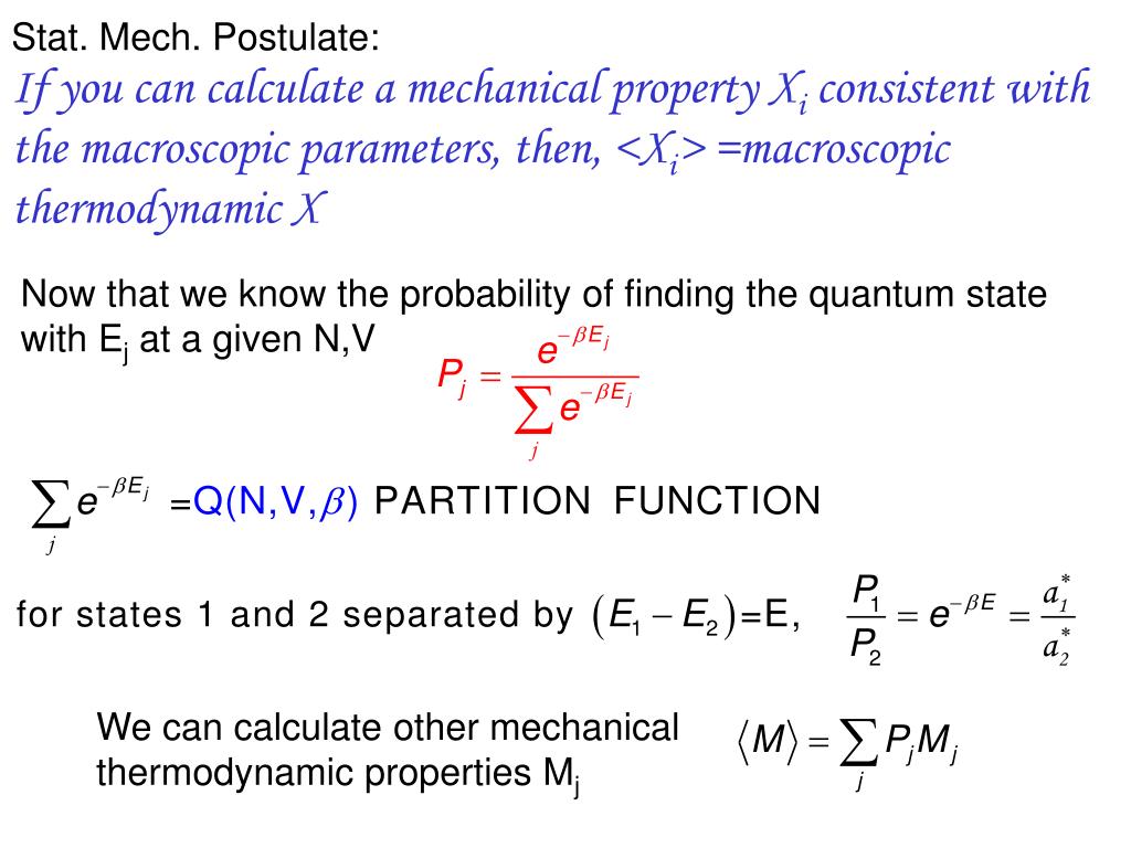
We can calculate other mechanical thermodynamic properties M j. Stat. Mech. Postulate: If you can calculate a mechanical property X i consistent with the macroscopic parameters, then, <X i > =macroscopic thermodynamic X. Using the postulate.
Using the postulate - slide 1
01 / 13Using the postulate
1 / 17

Télécharger la présentation

Using the postulate
Une image / un lien ci-dessous est fourni (tel quel) pour télécharger la présentation

Politique de téléchargement : le contenu du site vous est fourni TEL QUEL pour votre information et votre usage personnel ; il ne peut être vendu, concédé sous licence ni partagé sur d’autres sites sans l’accord de son auteur.Le contenu vous est fourni TEL QUEL, pour votre information et votre usage personnel uniquement. Téléchargez la présentation en cliquant sur ce lien. Lors du téléchargement, si vous ne parvenez pas à télécharger une présentation, l’éditeur a peut-être supprimé le fichier de son serveur.Pendant le téléchargement, si vous ne parvenez pas à obtenir une présentation, le fichier a peut-être été supprimé par l’éditeur.

F I N

Plus de contenu associé

Transcription de la présentation
  1. We can calculate other mechanical thermodynamic properties Mj Stat. Mech. Postulate: If you can calculate a mechanical property Xi consistent with the macroscopic parameters, then, <Xi> =macroscopic thermodynamic X Using the postulate Now that we know the probability of finding the quantum state with Ej at a given N,V

  2. Internal Energy

  3. Going back to the calculation of mechanical properties… Pressure With these tools in hand , we can now combine mechanical properties with thermodynamics and extract information about nonmechanical functions (like S or T)

  4. A A A A A B B B B B heat bath(T) Consider 2 ensembles A and B that become in thermal contact, with no change in volume  dV = 0 ; dA = 0 dB = 0 Derivation of b Initially W({a,b}) = W({a*}) x W({b*}) Ensemble A  bA Ensemble B  bB What are the b values at the new equilibrium?

  5. Derivation of b II

  6. dlnW=bdE

  7. The sum of the changes in energy in each system yields the infinitesimal change in the total energy

  8. Derivation of b Approaching equilibrium, there is an increase in the value of EA, heat is transferred from B to A. bA>bB At equilibrium bA =bB any change in W({a}) will be canceled by a similar change in W({b}) 1st law: equilibrium means TA =TB, and approaching equilibrium heat will be transferred from B to A when TA<TB

  9. and since and we obtain heatrev exchange workrev E and p relations

  10. From thermodynamics, we already know that or Gibbs Entropy Entropy

  11. and A(N,V,T)

  12. All relationships

  13. in the limit of T0 So far we worked with energy states, but we can easily change to levels, by counting how many times each “state” is repeated  degeneracy= W(N,V) States vs levels in the limit of T  Q(N,V,T)  constant = number of states