Capital Allocation and Profitability

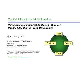
1. Risk Capital Strategy Value Capital Allocation and Profitability Using Dynamic Financial Analysis to Support Capital Allocation & Profit Measurement March 9/10, 2000 Manuel Almagro, FCAS, MAAA Principal Tillinghast - Towers Perrin This document is incomplete without the accompanying discussion; it is confidential and intended solely for the information and benefit of the immediate recipient thereof.

2. Capital can be allocated to business segment using the “expected policyholder deficit” measure • Expected policyholder deficit (EPD) = Expected (liabilities in excess of assets) • In this simple example, there is a 10% chance that losses will be $6,000; an 80% chance that losses will be $10,000; and a 10% chance that losses will be $14,000 • Assets are only $13,000, so there is a 10% chance of ruin, in which case the available $13,000 will be paid, leaving a deficit of $1,000 • Thus, at the funding ratio of 130%, the EPD ratio is 1% (both percentages are with respect to the expected losses of $10,000) 2

3. While the EPD illustration on the previous page is highly simplistic,the concepts readily generalize to more “real-world” situations • The illustration is intended only to show the conceptual essence of the insurance transaction • Policyholders and shareholders each contribute assets towards the funding of the liabilities • Policyholders contribute premiums based on expected loss costs and compensation for risk, based on market pricing • Shareholders contribute capital for the balance, to achieve the target overall funding ratio necessary to offer policyholders adequate security • Claims “happen”, and the assets are distributed • Claims are paid, up to the available assets • Shareholders receive the residual assets, if any, as their return • The split of assets between policyholder-supplied funds (premium) and shareholder-supplied funds (capital) is not necessary to the approach • The premium would reflect the expected losses of 10,000, plus a market determined return for risk-taking • Ignoring the return for risk, the premium would be 10,000 and the 130% funding ratio is equivalent to a 3.33:1 premium-to-surplus ratio

4. There are well-constructed theoretical arguments for the use of expected policyholder deficit in capital allocation • The EPD concept is taken from Risk-Based Capital development work (see Butsic’s paper in the 1994 Journal of Risk and Insurance) • EPD is different from ruin probability, because it takes into account the severity, as well as the frequency of ruinous scenarios • EPD takes the policyholder perspective – it recognizes that capital is there to provide security, and that the perceived level of security relates both to the potential frequency and severity of non-performance • Allocation on this basis is “fair" to policyholders — since they all have equal access to the entire base of capital, they are all receiving the same level of security – allocating capital based on EPD “charges them” equitably for the capital needed to create that level of security • The EPD is financially equivalent to the expected value of the shareholders’ option to “put" the company to the regulators if the liabilities exceed the available assets • In such instances the liabilities in excess of the assets would have to be paid by the Guaranty Funds – thus, EPD is also theoretically equivalent to the expected Guaranty Fund assessment 4

5. To illustrate the use of EPD in capital allocation, consider a two line example • As a starting point, each line has the same funding ratio of 130% • Each line also has the same 10% ruin probability • Because their risk profiles are different, the lines currently have different EPD ratio’s Product A Assets Probability Liabilities Payment Deficit Scenario 1 13,000 10.0% 6,000 6,000 0 Scenario 2 13,000 80.0% 10,000 10,000 0 Scenario 3 13,000 10.0% 14,000 13,000 1,000 Expected 13,000 100.0% 10,000 9,900 100 130.0% 1.0% Product B Assets Probability Liabilities Payment Deficit Scenario 1 13,000 10.0% 6,000 6,000 0 Scenario 2 13,000 80.0% 9,250 9,250 0 Scenario 3 13,000 10.0% 20,000 13,000 7,000 Expected 13,000 100.0% 10,000 9,300 700 130.0% 7.0% 5

6. If the two lines are independent, a company writing both lines would have an overall risk profile reflecting their convolution • At the current funding ratio of 130%, the combined lines have an expected deficit ratio of 2.0%; and the probability of ruin is 9% • If the company’s risk-capital constraint allowed only a 1% chance of ruin, additional assets of $4,000 would be required 6

7. The first step is to determine the required overall capital that satisfies all risk-capital constraints • A funding ratio of 150% is required to reduce the probability of ruin to the threshold level of 1% • After this risk-capital constraint is met, the overall EPD ratio is .20% 7

8. Having determined the overall level of required capital, the second step is to allocate the capital to business segment • The total assets of $30,000 are allocated such that the EPD ratio is the same for each product • Since Product B has larger potential losses, it has a higher funding ratio • While the overall EPD ratio is .2%, the line EPD ratios are both 2.0% 8

9. At EPD of .20% Marginal Net Funding Required Covariance Line Required Product Ratio Assets Benefit Allocation Assets A 15,800 5,400 3,240 12,560 158.0% B 22,800 1,800 1,080 21,720 228.0% C 16,800 1,800 1,080 15,720 168.0% Total 55,400 9,000 5,400 50,000 A B 35,000 34,280 U 175.0% A C 29,000 28,280 U 145.0% B C 39,600 37,440 U 198.0% A B C 50,000 50,000 U U 166.7% When there are more than two products, with different covariances, the allocation of the benefit requires a marginal analysis • To illustrate, consider a three product example in which the results for Product A are independent of the results for Products B and C, but the results for Products B and C are 100% correlated. The 1% ruin standard implies a corporate EPD of .20%. The total covariance benefit is 5,400, which is allocated based on a comparison of the marginal decrease in required assets when each product is added in to the other business • For example, Products B and C require assets of 39,600. When A is added in the total requirement drops from 55,400 to 50,000, for a marginal benefit of 5,400

10. The illustration demonstrates a workable approach to capital allocation • In summary, the capital allocation steps are as follows: • Set risk-capital constraints • Determine overall required assets and capital to meet all constraints • Translate overall required capital into implied EPD ratio • Calculate capital required by each line standing alone at constant EPD ratio • Determine overall covariance benefit across lines • Allocate covariance benefit based on marginal contribution of each line • The basic approach can be extended to incorporate other risks, and more realistic scenarios • Expenses, investment income, income taxes • Multiple accounting periods, timing of cash flows • Asset uncertainty • Accounting valuation rules, affecting the timing of the recognition of revenue, expense, and profit

11. Once the capital is allocated to a segment using the EPD approach, performance can be judged on an ROCE basis • A major benefit of the exercise is the ability to measure the returns on the capital employed by each segment, and to gauge the returns in relation to their risk • Returns in this context are the notional shareholder distributions, reflecting the investment of capital into the segment, and the release of that capital back to shareholders • Returns are measured on an economic, rather than a reported basis • This approach is consistent with actuarial appraisal theory, which measures economic values in the essentially the same manner • In addition to the expected results, the financial model produces a distribution of results – that distribution can be converted to a distribution of returns • Risk/return tradeoffs can be made by comparing expected ROCE to ROCE volatility • Rather than using standard deviation as the risk measure, a measure that emphasizes downside potential (below selected threshold) should be used ROCE - Return on Capital Employed, or return on allocated capital 11

12. To measure the riskiness of returns, we suggest using “Below Target Risk”, rather than standard deviation • The use of standard deviation as a measure of risk has been criticized • Standard deviation is a statistical measure of dispersion from the mean, which is not necessarily the same as risk • Standard deviation gives the same weight to dispersion below the mean as dispersion above the mean - a risk-averse person would place greater weight on the downside than the upside • Below Target Risk is computed in the same manner as a standard deviation, except • Deviations are measured from the “target”, which can be the mean or some other selected value reflecting the company’s “threshold for pain” • Only results below “target” are included in the calculations - deviations above the target are ignored • If the distribution is symmetric and the mean is chosen as the target, then the BTR will be one-half of the standard deviation • BTR =

13. The advantage of Below Target Risk over standard deviation can be illustrated by an example • These two return probability distributions have the same expected return of 13%, and the same standard deviation. • The top return distribution is clearly preferable to the bottom, as it has more upside, and less downside • Using a target return of 13%, the top distribution has a BTR of 23.5%; the bottom distribution has a BTR of 32.5% • Using a target return of 3% (roughly equivalent to a zero real return), the top distribution has a BTR of 17.6%; the bottom distribution has a BTR of 27.7% Probability Rate of Return 13%

14. Professional Liability Return Distribution 100% 80% 60% 40% 20% Rate of Return 0% -20% -40% -60% -80% -100% Cumulative Probability Distributions of results can be translated into distributions of returns on capital EXAMPLE

15. The adequacy of returns can then be judged in relation to risk • Risk to investors is measured by Below Target Risk as a proxy for systematic risk Security Market Line 18% Illustrative 14% Personal Automobile Expected Return 10% Large Cap Stock Small Cap Stock Real Estate Homeowners Bond Index Long Bond 6% Cash 2% 0.0% 4.0% 8.0% 12.0% 16.0% Below Target Risk (Negative Real Return)