Download
1 / 24
240 likes | 331 Vues
Explore the flows of costs and benefits over time to make informed investment choices based on intertemporal time preferences and interest rates. Learn how to analyze different investment options and their impact on net benefits.

E N D
Time and the Discount Rate • Project flows of costs and benefits are not even over time.
Option1 Year Cost Benefit Net 1 100 0 -100 2 10 0 -10 3 10 150 140 Sum 120 150 30 Option 2 Year Cost Benefit Net 1 40 50 10 2 40 50 10 3 40 50 10 Sum 120 150 30 Flow of Costs and Benefits Consider 2 Investment Options
Flow of Costs and Benefits Net Benefits by Year
Flow of Costs and Benefits • These two options have very different flows of costs and benefits over time. • Is there any difference between these two options? • Which is preferred?
Flow of Costs and Benefits • In order to address this question, need to understand how the future is valued relative to the present: • Intertemporal time preferences • The interest rate
Time Preference of Consumers • Consider consumers have a stock of wealth today, and must choose to consume between today and tomorrow. • Intertemporal indifference map • Time indifference • Intertemporal indifference curve
Intertemporal Consumption Choice Consumption T1 x S1 x I0 (Intertemporal Indifference Curve) S0 C1 C0 Consumption T0
Intertemporal Consumption Choice A Family of Indifference Curves Consumption T1 Consumption T0
Time Preference of Consumers • Expect consumers to have “positive time preference” : • prefer consumption today rather than in the future • Why? • There is a chance that will not be able to consume in the future • (in the long run we are all dead) • Expectation that income will be higher in the future (economy will grow) • (Goods and services will be more abundant in the future as a result of economic growth)
Intertemporal Consumption Choice Consumption T1 “PPF” (Slope=-1) S0 = C0 Se < Ce Zero time preference Positive time preference 450 Ce C0 Consumption T0
The price of current consumption • Income or wealth that is consumed today is not available to be saved for consumption in the future. • What is the price of consuming today? • Interest rate: amount that savings today can be increased in the future, through investment.
Interest Rate • The price (or opportunity cost) of consuming a dollar of income or wealth today rather than saving for consumption in the future • Expressed as a percentage increase: • (K1/K0)-1} * 100 K0 money invested in time 0 K1 money obtained from investment in time 1
Interest Rate • Example: • Invest $100 in time 0 • Return = $112 in time 1 • Interest rate= (112/100-1) * 100 = 12% • A unit-free measure, expressed as a ratio
Interest Rate Consumption T1 150 112 100 i = 50% i = 12% i = 0% 100 Consumption T0
Time Preference of Consumers • From consumers’ time preferences, derive the supply of savings. Determine amount of income and wealth that households will save for the future at different interest rates.
Response to change in interest rate Consumption T1 i2 i1 S2 S1 i0 S0 Consumption T0
Response to change in interest rate Interest Rate Ssavings i2 x x i1 i0 x S0 S1 S2 Savings ($)
Investment opportunities • Investment opportunities generate the demand for savings (capital) • Intertemporal production possibility frontier
Intertemporal production possibility frontier Production1 I1 PPF I0 P1 P0 Production0
Demand for Investment • Rank potential investments according to the rate of return, from highest to lowest. • This will give the derived demand schedule for savings
Demand for Investment Production1 i2 i2 I1 i1 I0 PPF i0 Production0
Response to change in Interest Rate Interest Rate i0 x x i1 i2 x Demand for Invesment I0 I1 I2 Investment Demand ($)
Capital Market Supply of Savings i ieq Demand for Investment Qeq Quantity ($)
Interest rate • In market equilibrium • interest rate (r) = MRS = MRT • In reality: transactions costs associated with matching up suppliers and demanders of savings: • Financial intermediation (banks) • Spread between savings and borrowing rate • Risk premia