Download
1 / 70
720 likes | 913 Vues
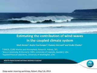
Estimating the contribution of wind-waves in the coupled climate system. Mark Hemer 1 , Baylor Fox-Kemper 2 , Ramsey Harcourt 3 and Elodie Charles 1 1 CAWCR, CSIRO Marine and Atmospheric Research, Hobart, TAS. 2 Brown University, RI (formerly CIRES, University of Colorado, Boulder), USA.

E N D
Estimating the contribution of wind-waves in the coupled climate system Mark Hemer1, Baylor Fox-Kemper2, Ramsey Harcourt3 and Elodie Charles1 1CAWCR, CSIRO Marine and Atmospheric Research, Hobart, TAS. 2 Brown University, RI (formerly CIRES, University of Colorado, Boulder), USA. 3 Applied Physical Laboratory, University of Washington, USA. Wealth from Oceans National Research Flagship Deep-water mooring workshop, Hobart, May 5-6, 2014.
Presentation Outline • Introduction/Motivation • Methodology • Mixing models • PWP with Langmuir • SMC with Langmuir • Model Forcing • Atmospheric • Wave • Model initialisation and integration • Results • Ongoing Work/Concluding Remarks • If time, consideration of contribution wave drag effects on global flux estimates
The contribution of:Wave-driven mixing of the Surface Mixed LayerIntroduction
Air-Sea flux biases in AOGCMs (e.g., CCSM3/4) Qa SW Latent Total flux CCSM3 Bias CCSM4 Bias Bates et al., 2012.
Wind and waves not in equilibrium • Swell dominates global wave field. (Fan et al., 2014) • Global distribution of fraction of wave energy which is swell
The contribution of:Wave-driven mixing of the Surface Mixed LayerMethodology: Mixing Models
Wave driven surface ocean mixing: 3 possible processes Injection of turbulence by breaking waves. Mixes to depth approximately equal to the wave height (Craig and Banner, 1994) Langmuir mixing mixes to a depths of order 100m. (Langmuir, 1938) Non-breaking wave mixing. It has been proposed turbulence generated by wave orbital motion can mix to depths of order 100m. (Babanin, 2006)
August Southern Ocean mixed layer bias (Webb et al., 2010) Wave dependent mixing Dong et al. Observations CCSM3.5 with Langmuir CCSM3.5 Control without Langmuir
Langmuir Parameterisation in mixing models • Bulk Model • Price-Weller-Pinkel model with amended Li and Garrett (1995) Langmuir parameterisation • Profile Models • Second-moment-closure (following Mellor-Yamada) with Langmuir Parameterisation (Harcourt, 2012) • Alternate tunings • E6=7 (tuning to minimise error in prediction of TKE levels) • E6=5 (tuning to predict vertical TKE to compare with vertical float m’ments) • GV=GS=0 (Reduction to Kantha and Clayson, 2004) • K-Profile Parameterisation of Langmuir turbulence (McWilliams, 2000; Smyth, 2002; McWilliams, 2012; Fan and Griffies, 2014)
Langmuir Parameterisation in mixing models • Bulk Model • Price-Weller-Pinkel model with amended Li and Garrett (1995) Langmuir parameterisation • Profile Models • Second-moment-closure (following Mellor-Yamada) with Langmuir Parameterisation (Harcourt, 2012) • Alternate tunings • E6=7 (tuning to minimise error in prediction of TKE levels) • E6=5 (tuning to predict vertical TKE to compare with vertical float m’ments) • GV=GS=0 (Reduction to Kantha and Clayson, 2004) • K-Profile Parameterisation of Langmuir turbulence (McWilliams, 2000; Smyth, 2002; McWilliams, 2012; Fan and Griffies, 2014)
Price-Weller-Pinkel mixed layer model (Price et al., 1986) Wind Stress and Heat Flux Static instability mixing Bulk Richardson instability mixing Shear instability mixing Redistributions of T, S, r and U Mixed layer depth Vertical profile of horizontal velocity Vertical profile of T, S and r
Incorporation of LC into the PWP model (Li et al.,1995) Langmuir cells penetration depth depends on competition between vertical motion and stratification, represented by the Froude number. Vertical penetration is inhibited when Fr reaches a critical value Frc = 0.6 (LG97). This was parameterised by Li and Garret using: (after LG93) This gives an additional stability criteria (i.e., that deepening of the SML will not occur if) Under the assumption of a fully developed sea.
Amended Fr scaling of Langmuir Mixing in PWP Flor et al. (2010) suggest wdn = 5.2wrms, so Froude based stability criteria becomes: wrmsobtained from LES model scaling (Van Roekel et al., 2012): , where c1= 1.5 and c2=5.4. For the case where wind and waves are non-aligned, a = angle b/w wind and langmuir cell direction, qwwis angle b/w stokes drift and wind.
PWP mixed layer model with LC parameterisation Wind Stress and Heat Flux Static instability mixing Bulk Richardson instability mixing Shear instability mixing Langmuir mixing Redistributions of T, S, r and U Mixed layer depth Vertical profile of horizontal velocity Vertical profile of T, S and r
Second moment closure model with langmuirparamn(Harcourt, 2013) Turbulent Kinetic Energy Equation PS = Shear Production Pb = Buoyancy Flux Harcourt (2013) modifies for impact of Craik-Leibovich vortex forcing using
Harcourt SMC model with langmuir turbulence (2013, JPO) CL vortex force (Craik and Leibovich, 1976) included in momentum equation after McWilliams et al (1997): uj is surface-wave phase-averaged Eulerian velocity, ujS is the surface wave Stokes drift, P is non-hydrostatic pressure, r0 is reference density, fkis Coriolis components, gk is gravitational acceleration, n is viscosity q is a thermodynamic scalar with expansion coefficient a and diffusivity kq. Deriving Reynolds stress and flux equations for fluctuations uj’, q’and a slowly- or non-fluctuating Stokes drift gives: Kantha and Clayson (2004) included this production term
The contribution of:Wave-driven mixing of the Surface Mixed LayerMethodology: Model Forcing
Large and Yeager (2004) CORE normal year forcing Standard air-sea flux dataset of WGOMD Coupled Ocean-Ice Reference Experiment Atmospheric Fields • ISCCE: Daily varying shortwave and longwaveradiative fluxes (no diurnal cycle) • NCEP/NCAR: Six-hourly varying meteorological fields (1948-2006) 10m TA, humidity, zonal/ meridional winds, SLP • GCGCS: Annual mean river runoff • GCGCS: Monthly varying precipitation (12 time steps per year) Large and Yeager (2004, 2009) Bulk Formula • Sfc BC determines fluxes of heat, freshwater and momentum • Net heat flux = Sensible + Latent + Shortwave + Longwave • Net freshwater flux = Precip – Evap + River Runoff • Net momentum exchange is driven by windstress Large and Yeager (2004) Solution set • Solves bulk formula under CORE forcing using Hadley OI-SST
Large and Yeager (2004) CORE normal year forcing Standard air-sea flux dataset of WGOMD Coupled Ocean-Ice Reference Experiment Atmospheric Fields • ISCCE: Daily varying shortwave and longwaveradiative fluxes (no diurnal cycle) • NCEP/NCAR: Six-hourly varying meteorological fields (1948-2006) 10m TA, humidity, zonal/ meridional winds, SLP • GCGCS: Annual mean river runoff • GCGCS: Monthly varying precipitation (12 time steps per year) Large and Yeager (2004, 2009) Bulk Formula • Sfc BC determines fluxes of heat, freshwater and momentum • Net heat flux = Sensible + Latent + Shortwave + Longwave • Net freshwater flux = Precip – Evap + River Runoff • Net momentum exchange is driven by windstress Large and Yeager (2004) Solution set • Solves bulk formula under CORE forcing using Hadley OI-SST
CORE normal year consistent wave field WaveWatch III (v4.08) CORE normal year winds forcing. 1° spatial resolution 13 month integration: (dec) spinup + 1 whole CORE normal yr. Full directional spectra archived 6-hourly at 4 ° resolution.
Model Initialisation: Real ARGO profile. Most representative summer solstice (shallow MLD) profile (taken within 1.5° radius of wave archive location, +/- 20 days from summer solstice date. Depth (m) Temperature (°C)
Model Forcing: CORE Normal Year (Large and Yeager, 2004). Bulk fluxes, using evolving mixing model SST • •Daily varying shortwave and longwaveradiative fluxes (no diurnal cycle) • •Six-hourly varying meteorological fields (1948-2006) • 10m TA, humidity, zonal/ meridional winds, SLP • Annual mean river runoff • •Monthly varying precipitation (12 time steps per year) • Six-hourly varying stokes velocity profile from CORE forced wave model 1-D Mixing Model: Harcourt (2012): SMC with Langmuir Summer Solstice Depth (m) Temperature (°C) Model applied with zero waves (solid) and COREwave (dashed) fields
Model Forcing: CORE Normal Year (Large and Yeager, 2004). Bulk fluxes, using evolving mixing model SST • •Daily varying shortwave and longwaveradiative fluxes (no diurnal cycle) • •Six-hourly varying meteorological fields (1948-2006) • 10m TA, humidity, zonal/ meridional winds, SLP • Annual mean river runoff • •Monthly varying precipitation (12 time steps per year) • Six-hourly varying stokes velocity profile from CORE forced wave model 1-D Mixing Model: Harcourt (2012): SMC with Langmuir Depth (m) Temperature (°C) Model applied with zero waves (solid) and COREwave (dashed) fields
Model Forcing: CORE Normal Year (Large and Yeager, 2004). Bulk fluxes, using evolving mixing model SST • •Daily varying shortwave and longwaveradiative fluxes (no diurnal cycle) • •Six-hourly varying meteorological fields (1948-2006) • 10m TA, humidity, zonal/ meridional winds, SLP • Annual mean river runoff • •Monthly varying precipitation (12 time steps per year) • Six-hourly varying stokes velocity profile from CORE forced wave model 1-D Mixing Model: Harcourt (2012): SMC with Langmuir Depth (m) Temperature (°C) Model applied with zero waves (solid) and COREwave (dashed) fields
Model Forcing: CORE Normal Year (Large and Yeager, 2004). Bulk fluxes, using evolving mixing model SST • •Daily varying shortwave and longwaveradiative fluxes (no diurnal cycle) • •Six-hourly varying meteorological fields (1948-2006) • 10m TA, humidity, zonal/ meridional winds, SLP • Annual mean river runoff • •Monthly varying precipitation (12 time steps per year) • Six-hourly varying stokes velocity profile from CORE forced wave model 1-D Mixing Model: Harcourt (2012): SMC with Langmuir Summer Depth (m) Temperature (°C) Model applied with zero waves (solid) and COREwave (dashed) fields
Model Forcing: CORE Normal Year (Large and Yeager, 2004). Bulk fluxes, using evolving mixing model SST • •Daily varying shortwave and longwaveradiative fluxes (no diurnal cycle) • •Six-hourly varying meteorological fields (1948-2006) • 10m TA, humidity, zonal/ meridional winds, SLP • Annual mean river runoff • •Monthly varying precipitation (12 time steps per year) • Six-hourly varying stokes velocity profile from CORE forced wave model 1-D Mixing Model: Harcourt (2012): SMC with Langmuir Summer Depth (m) Temperature (°C) Model applied with zero waves (solid) and COREwave (dashed) fields
Model Forcing: CORE Normal Year (Large and Yeager, 2004). Bulk fluxes, using evolving mixing model SST • •Daily varying shortwave and longwaveradiative fluxes (no diurnal cycle) • •Six-hourly varying meteorological fields (1948-2006) • 10m TA, humidity, zonal/ meridional winds, SLP • Annual mean river runoff • •Monthly varying precipitation (12 time steps per year) • Six-hourly varying stokes velocity profile from CORE forced wave model 1-D Mixing Model: Harcourt (2012): SMC with Langmuir Summer Depth (m) Temperature (°C) Model applied with zero waves (solid) and COREwave (dashed) fields
Model Forcing: CORE Normal Year (Large and Yeager, 2004). Bulk fluxes, using evolving mixing model SST • •Daily varying shortwave and longwaveradiative fluxes (no diurnal cycle) • •Six-hourly varying meteorological fields (1948-2006) • 10m TA, humidity, zonal/ meridional winds, SLP • Annual mean river runoff • •Monthly varying precipitation (12 time steps per year) • Six-hourly varying stokes velocity profile from CORE forced wave model 1-D Mixing Model: Harcourt (2012): SMC with Langmuir Summer Depth (m) Autumn Temperature (°C) Model applied with zero waves (solid) and COREwave (dashed) fields
Model Forcing: CORE Normal Year (Large and Yeager, 2004). Bulk fluxes, using evolving mixing model SST • •Daily varying shortwave and longwaveradiative fluxes (no diurnal cycle) • •Six-hourly varying meteorological fields (1948-2006) • 10m TA, humidity, zonal/ meridional winds, SLP • Annual mean river runoff • •Monthly varying precipitation (12 time steps per year) • Six-hourly varying stokes velocity profile from CORE forced wave model 1-D Mixing Model: Harcourt (2012): SMC with Langmuir Summer Depth (m) Autumn Temperature (°C) Model applied with zero waves (solid) and COREwave (dashed) fields
Model Forcing: CORE Normal Year (Large and Yeager, 2004). Bulk fluxes, using evolving mixing model SST • •Daily varying shortwave and longwaveradiative fluxes (no diurnal cycle) • •Six-hourly varying meteorological fields (1948-2006) • 10m TA, humidity, zonal/ meridional winds, SLP • Annual mean river runoff • •Monthly varying precipitation (12 time steps per year) • Six-hourly varying stokes velocity profile from CORE forced wave model 1-D Mixing Model: Harcourt (2012): SMC with Langmuir Summer Depth (m) Autumn Temperature (°C) Model applied with zero waves (solid) and COREwave (dashed) fields
Model Forcing: CORE Normal Year (Large and Yeager, 2004). Bulk fluxes, using evolving mixing model SST • •Daily varying shortwave and longwaveradiative fluxes (no diurnal cycle) • •Six-hourly varying meteorological fields (1948-2006) • 10m TA, humidity, zonal/ meridional winds, SLP • Annual mean river runoff • •Monthly varying precipitation (12 time steps per year) • Six-hourly varying stokes velocity profile from CORE forced wave model 1-D Mixing Model: Harcourt (2012): SMC with Langmuir Summer Depth (m) Autumn Winter Temperature (°C) Model applied with zero waves (solid) and COREwave (dashed) fields
Model Forcing: CORE Normal Year (Large and Yeager, 2004). Bulk fluxes, using evolving mixing model SST • •Daily varying shortwave and longwaveradiative fluxes (no diurnal cycle) • •Six-hourly varying meteorological fields (1948-2006) • 10m TA, humidity, zonal/ meridional winds, SLP • Annual mean river runoff • •Monthly varying precipitation (12 time steps per year) • Six-hourly varying stokes velocity profile from CORE forced wave model 1-D Mixing Model: Harcourt (2012): SMC with Langmuir Summer Depth (m) Autumn Winter Temperature (°C) Model applied with zero waves (solid) and COREwave (dashed) fields
Model Forcing: CORE Normal Year (Large and Yeager, 2004). Bulk fluxes, using evolving mixing model SST • •Daily varying shortwave and longwaveradiative fluxes (no diurnal cycle) • •Six-hourly varying meteorological fields (1948-2006) • 10m TA, humidity, zonal/ meridional winds, SLP • Annual mean river runoff • •Monthly varying precipitation (12 time steps per year) • Six-hourly varying stokes velocity profile from CORE forced wave model 1-D Mixing Model: Harcourt (2012): SMC with Langmuir Summer Depth (m) Autumn Winter Temperature (°C) Model applied with zero waves (solid) and COREwave (dashed) fields
Model Forcing: CORE Normal Year (Large and Yeager, 2004). Bulk fluxes, using evolving mixing model SST • •Daily varying shortwave and longwaveradiative fluxes (no diurnal cycle) • •Six-hourly varying meteorological fields (1948-2006) • 10m TA, humidity, zonal/ meridional winds, SLP • Annual mean river runoff • •Monthly varying precipitation (12 time steps per year) • Six-hourly varying stokes velocity profile from CORE forced wave model 1-D Mixing Model: Harcourt (2012): SMC with Langmuir Summer Depth (m) Autumn Winter Spring Temperature (°C) Model applied with zero waves (solid) and COREwave (dashed) fields
Harcourt SMC NO WAVESWAVES ARGO PROFILES 50N, 145W
Experiments carried out • Carry out annual integration at each location we have spectral wave data archived (globally on 4° grid) • Repeat computations with alternative mixing schemes • Harcourt (2012) SMC with langmuir parameterisation • Alternate tunings • E6=7 (tuning to minimise error in prediction of TKE levels) • E6=5 (tuning to predict vertical TKE to compare with vertical float m’ments) • GV=GS=0 (Reduction to Kantha and Clayson, 2004) • Price-Weller-Pinkel model with amended Li and Garrett (1995) Langmuir parameterisation
The contribution of:Wave-driven mixing of the Surface Mixed LayerResults
Percentage increase in MLD with introduction of SMC (E6=7) langmuir mixing ~180 days after Summer Solstice Zonal mean MLD after 180days after 365 days
Annual Cycle (PAPA) Mean wave flux is ~0.3 Wm-2 WAVES NO WAVES 7 Wm-2
Annual Mean Surface Heat Flux Equivalent with addition of Langmuir mixing (Wm-2) E6=7
Implied Annual Mean Northward Heat Transport (Wm-2) Watts Global equivalent bias ~11.5Wm-2 ~8.6Wm-2 NO WAVES WAVES SMC Langmuir implies ocean stores an extra 1.0PW Latitude Note: Plot not directly comparable to Atm flux calcs. Can not assume that storage is uniformally distributed, as 1d model with/without waves is calculating spatial distribution of storage. If we remove this influence (by the above assumption applied previously to ensure convergence to zero at Northern boundary), the lines overlay one another.
Percentage increase in MLD with introduction of SMC (E6=5) langmuir mixing ~180 days after Summer Solstice Zonal mean MLD after 180days after 365 days
Percentage increase in MLD with introduction of SMC (E6=7) langmuir mixing ~180 days after Summer Solstice Reduced to Kantha&Clayson Approximation GV=GS=0 Zonal mean MLD after 180days after 365 days
PWP-Lc NO WAVESWAVES ARGO PROFILES 50N, 145W
Percentage increase in MLD with introduction of PWP langmuir mixing ~180 days after Summer Solstice Zonal mean MLD after 180days after 365 days
Summarising the contribution of langmuirparameterisation in mixing models c.f., annual mean global energy flux from wind-waves = 70TW annual mean global energy flux from waves-OML= 68TW (Rascle et al., 2008)
The contribution of:Wave-driven mixing of the Surface Mixed LayerOngoing work/Concluding remarks