Interlude (Optimization and other Numerical Methods)
Interlude (Optimization and other Numerical Methods). Fish 458, Lecture 8. Numerical Methods.

Interlude (Optimization and other Numerical Methods)
E N D
Presentation Transcript
Interlude(Optimization and other Numerical Methods) Fish 458, Lecture 8
Numerical Methods • Most fisheries assessment problems are mathematically too complicated to apply analytical methods. We often have to resort to numerical methods. The two most frequent questions requiring numerical solutions are: • Find the values for a set of parameters so that they satisfy a set of (non-linear) equations. • Find the values for a set of parameters to minimize some function. • Note:Numerical methods can (and do) fail – you need to know enough about them to be able to check for failure.
Minimizing a Function • The problem: • Find the vector so that the function is minimized (note: maximizing is the same as minimizing ). • We may place bounds on the values for the elements of (e.g. some must be positive). • By definition, for a minimum:
Analytic Approaches • Sometimes it is possible to solve the differential equation directly. For example: • Now:
Linear Models – The General Case • Generalizing: • The solution to this case is: • Exercise: check it for the simple case:
Analytical Approaches-II • Use analytical approaches whenever possible. Finding analytical solutions for some of the parameters of a complicated model can substantially speed up the process of minimizing the function. • For example: q for the Dynamic Schaefer model:
Numerical Methods (Newton’s Method)Single variable version-I • We wish to find the value of x such that f(x) is at a minimum. • Guess a value for x • Determine whether increasing or decreasing x will lead to a lower value for f(x) (based on the derivative). • Assess the slope and its change (first and second derivatives of f) to determine how far to move from the current value of x. • Change x based on step 3. • Repeat steps 2-4 until no further progress is made.
Numerical Methods (Newton’s Method)Single variable version-II • Formally: • Note: Newton’s method may diverge rather than converge!
Minimize: 2+(x-2)^4-x^2 This is actually quite a nasty function – differentiate it and see! Minimum: -6.175 at x = 3.165 Convergence took 17 steps in this case.
Numerical Methods (Newton’s Method) • If the function is quadratic (i.e. the third derivative is zero), Newton’s method will get to the solution in one step (but then you could solve the equation by hand!) • If the function is non-quadratic, iteration will occur. • Multi-parameter extensions to Newton’s method exist but most people prefer gradient free methods (e.g. SIMPLEX) to deal with problems like this.
Calculating Derivatives Numerically-I • Many numerical methods (e.g. Newton’s method) require derivatives. You should generally calculate the derivatives analytically. However, sometimes, this gets very tedious. For example, for the Dynamic Schaefer model: • I think you get the picture…
Calculating Derivatives Numerically-II • The accuracy of the approximation depends on the number of terms and the size of x / y (smaller – but not too small – is better)
Optimization – some problems-I • Local minima Global minimum Local minimum
Optimization – some problems-II • Problems calculating numerical derivatives. • Integer parameters. • Bounds [either on the function itself (extinction of Cape Hake hasn’t happened - yet) or on the values for the parameters].
Optimization – Tricks of the Trade-I • To keep a parameter,x, constrained between a and b, transform it to a+(0.5+arctan(y)/)(b-a). x=1+(0.5+arctan(y)/) x~[1-2]
Optimization – Tricks of the Trade-II • Test the code for the model by fitting to data where the answer is known! • Look at the fit graphically (have you maximized rather than minimizing the function)? • Minimize the function manually; restart the optimization algorithm from the final value; restart the optimization algorithm from different values. • When fitting n parameters that must add to 1, fit n-1 parameters and set the last to 1-sum(1:n-1). • In SOLVER, use automatic scaling and set the convergence criterion smaller.
Solving an Equation(the Bisection Method) • Often we have to solve the equation f(x)=0 (e.g. the Lokta equation). This can be treated as an optimization problem (i.e. minimize f(x)2). • However, it is usually more efficient to use a numerical method specifically developed for this purpose. • We illustrate the Bisection Method here but there are many others.
Solving an Equation(the Bisection Method) Find x such that 10+20(x-2)^3+100(x-2)^2=0
Note • Use of Numerical Methods (particularly optimization) is an art. The only way to get it right is to practice (probably more than anything else in this course).
Readings • Hilborn and Mangel (1997); Chapter 11 • Press et al. (1988), Chapter 10