STATISTICS

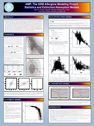
1. AMP: The GRB Afterglow Modeling Project Statistics and Extinction/Absorption Models Adam S. Trotter, Daniel E. Reichart & Andrew C. Foster University of North Carolina at Chapel Hill ABSTRACT AMP models extinction due to dust in source frame of the host galaxy and in the Milky Way using the near UV-Infrared extinction model of Cardelli, Clayton & Mathis (1989) [CCM] and the UV extinction model of Fitzpatrick & Massa (1988, 1990) [FM]. The extinction at a given source-frame wavelength lambda can be expressed as: The paramater AV normalizes the extinction curve in the V-band, and RV= AV /E(B-V) is a measure of the extintion in the B-band relative to the V-band. Extinction due to dust in the Milky Way is described by the CCM model, with a Gaussian prior logRV,MW = log(3.1) ± 0.1, and a fixed value of E(B-V)MW given by the model of Schlegel, Finkbeiner & Davis (1998). Extinction in the host galaxy is described by a combination of the CCM and FM models; the only free parameters are AV , and the CCM model parameters c2 and c4 . The other parameters in the model, including RV, are constrained by priors we obtained from analysis of published extinction measurements for 417 stars in the Milky Way (Valencic, Clayton & Gordon 2004) and 23 stars in the Large and Small Magellanic Clouds (Gordon et al. 2003). The extinction models and priors are summarized below. • The Afterglow Modeling Project (AMP) will determine, in a statistically self-consistent way, parameters that describe the time- and frequency-dependent emission and absorption of every gamma-ray burst (GRB) afterglow observed since the first detection in 1997, using all published data for each GRB. The result will be an ever-growing catalog of fitted model parameters for GRB afterglows that can itself be analyzed to better describe the range of and relationships among the physical properties of GRBs and their environments. We first present the Bayesian statistic we use to fit afterglow models. Our statistic corrects for inherent problems we have discovered in previous two-dimensional statistics. We then present the parameterized model for GRB afterglow extinction and absorption. Approximately 40 parameters describe line-of-sight extinction due to dust and absorption due to neutral hydrogen and molecular hydrogen in the GRB host galaxy; absorption due to neutral hydrogen in the intergalactic medium (the Lyα forest); and extinction due to dust in the Milky Way. This very large parameter space is significantly reduced by priors, which we determined by analyzing previously published extinction measurements of stars in our Galaxy, and flux deficits due to Lyman-alpha absorption in the spectra of quasars at redshifts in the range 2 < z < 6.5, which includes the Gunn-Peterson trough. The AMP project aside, these parameters and priors can be used to model extinction and absorption towards any extragalactic point source. Correlation between extinction parameters c1 and c2. Solid line is the best-fit linear model: Shaded regions are the 1, 2 and 3σ confidence intervals of the fit. Best fit parameters provide Gaussian priors: The reference value minimizes correlation between fitted parameters b and m. Correlation between UV bump height c3/γ2 and c2. Solid line is the best-fit smoothly-broken linear model Shaded regions are the 1, 2 and 3σ confidence intervals of the fit. Best fit parameters provide Gaussian priors: , . Reference values minimize correlations among fitted parameters. Correlation between extinction parameters RV and c2. Solid line is the best-fit smoothly-broken linear model Shaded regions are the 1, 2 and 3σ confidence intervals of the fit. Best fit parameters provide Gaussian priors: . Reference values minimize correlations among fitted parameters. DUST EXTINCTION MODEL • For source frame x = 1μm/λ< 1.82, we use the CCM extinction model: • where y = x – 1.82. • For 3.3 < x < 10.96, we use the FM extinction model: • For 1.82 < x < 3.3, we use a weighted average of the two models. For x > 10.96 (Lyman limit), absorption due to neutral hydrogen in the host galaxy is total (Aλ = ∞).In the AMP dust extinction model, c2, c4 and AV are free parameters; c1, UV bump height c3/γ2, and RV are constrained by priors on the correlation model parameters (see figures). γ and x0 are constrained by Gaussian priors whose widths σγ and σxo themselves have Gaussian priors: • AMP dust extinction model curve (Reichart 2001) STATISTICS Given a two dimensional data set of N points in the x-y plane with intrinsic uncertainties in both dimensions {xn,yn; σx,n,σy,n}, Bayes’ theorem allows us to compute the probability of a hypothetical model distribution, described by a curve defined by M parameters yc(x;θm) and extrinsic sample variance (σx,σy), given any prior constraints on the parameters. If we assume the intrinsic errors and sample variance have Gaussian probability distributions, and the prior distributions are flat, the best-fit model is found by maximizing the likelihood: where and For a given data point, the path integral along the curve yc is approximated by finding the point at which the curve is tangent to an ellipse with axes proportional to Σx, Σx, and integrating along a line through that point with slope mt (bottom right figure). The result of this integral depends upon the choice of the differential element ds. D’Agostini (2005) [D05] uses ds=dx. Reichart (2001) [R01] uses We present a new statistic [TRF09] where the differential element is projected onto a line perpendicular to the segment connecting the data point and the tangent point of the curve to the intrinsic error ellipse; the angle between this line and the tangent line is φ, where the tangent line has slope mt′ = tanθ′ (top right figure). Two criteria motivate our choice: 1) The statistic should invertible: i.e., if xn  yn and σxn σyn the best-fit model parameters should describe the curve xc (y) = yc-1 (x). 2) The statistic should reduce to the traditional 1D χ2 statistic when σx= 0 or σy= 0. Below is a summary of the properties of the D05, R01 and TRF09 statistics for the case of a linear model yc = mx + b. Note that for a linear model, mt= m′t= m. Top: model curve distribution and tangent line with respect to the intrinsic error ellipse of the data point. Bottom: After adding intrinsic and extrinsic errors in quadrature, the tangent line changes. Shaded areas indicate 1, 2 and 3σconfidence regions. The blue line provides the differential element for the likelihood function path integration. H2 ABSORPTION MODEL Linear fits to a symmetric Gaussian random distribution of width σ=1 in (x, y) of 1000 data points with small, random errorbars σx ≠ σy ≈ 0.01.Left: Fit to x vs. y using D05, R01 and TRF09 statistics. Center: Fits to y vs. x for the same data set. Note that the D05 and R01 fits are invertible (mxy=1/myx), while D05 is biased towards m=0 in both fits. Right: Probability distribution of θ = tan-1(m) for ensembles of fits to Gaussian random clouds of N=1000 points with symmetric errorbars σx= σy. pR01(θ)=pTRF09(θ)=constant, while pD05(θ)  cosNθ. Lyα FOREST MODEL • Theoretical absorption spectra due to rovibrationally excited molecular hydrogen for column densities NH2 =1016, 1018 and 1020 cm-2, for clouds fully shielded from (left) and exposed to (right) Lyman continuum radiation from the GRB (Draine 2000). For computational simplicity, we approximate these spectra with broken line absorption profiles (dashed lines). AMP models H2 absorption by interpolating between these broken lines, with column density NH2 and fractional Lyman continuum illumination 0 XLyc 1 as free parameters. • Lyα transmission T vs. absorber redshift z. Points are flux deficits for 64 QSOs, measured in binned regions of their spectra redward of Lyα in the source frame (Fan et al. 2006; Songaila 2004). The solid line is the best-fit to the model: • Shaded regions are the 1, 2 and 3σ confidence intervals of the fit. AMP models Lyα forest absorption using the parameters a, b, c, d and sample variance σz with Gaussian priors, along with a prior source redshift zGRB from spectral or other observations. IGM absorption model priors are: • The redshifts z1 = 3.8826 and z2 = 6.2279 were chosen to minimize correlations among fitted parameters. Note the onset of the Gunn-Peterson trough at z≈ 6. • The AMP model also includes a damped Lyman absorber profile at the source redshift, whose shape is parameterized by the neutral hydrogen column density NH, and total absorption at wavelengths shorter than the Lyman limit λ < 912Å in the source frame. NH may be fit as a free parameter, or with prior constraints from X-ray or other observations, when available. REFERENCES • Cardelli, J. A., Clayton, G. C. & Mathis, J. S. 1989. The Relationship between Infrared, Optical, and Ultraviolet Extinction. Astrophysical Journal 345:245-256. • D'Agostini, G. 2005. Fits, and Especially Linear Fits, with Errors on Both Axes, Extra Variance of the Data Points and Other Complications. arXiv:physics/0511182. [D05] • Draine, B. T. 2000. Gamma-Ray Bursts in Molecular Clouds: H2 Absorption and Fluorescence. Astrophysical Journal 532:273-280. • Fan, X., et al. 2006. Constraining the Evolution of the Ionizing Background and the Epoch of Reionization with z~6 Quasars. II. A Sample of 19 Quasars. Astronomical Journal 132:117-136. • Fitzpatrick, E. L. & Massa, D. 1988. An Analysis of the Shapes of Ultraviolet Extinction Curves. II - The Far-UV extinction. Astrophysical Journal 328:734-746. • Fitzpatrick, E. L. & Massa, D. 1990. An Analysis of the Shapes of Ultraviolet Extinction Curves. III - An Atlas of Ultraviolet Extinction Curves. Astrophysical Journal Supplement Series 72:163-189. • Gordon, K. D., Clayton, G. C., Misselt, K. A., Landolt, A. U. & Wolff, M. J. 2003. A Quantitative Comparison of the Small Magellanic Cloud, Large Magellanic Cloud, and Milky Way Ultraviolet to Near-Infrared Extinction Curves. Astrophysical Journal 594:279-293. • Reichart, D. E. 2001. Dust Extinction Curves and Lyα Forest Flux Deficits for Use in Modeling Gamma-Ray Burst Afterglows and All Other Extragalactic Point Sources. Astrophysical Journal 553:235-253. [R01] • Schlegel, David J., Finkbeiner, D. P. & Davis, M. 1998. Maps of Dust Infrared Emission for Use in Estimation of Reddening and Cosmic Microwave Background Radiation Foregrounds. Astrophysical Journal 500:525. • Songaila, A. 2004. The Evolution of the Intergalactic Medium Transmission to Redshift 6. Astronomical Journal 127:2598-2603. • Valencic, L. A., Clayton, G. C. & Gordon, K. D. 2004. Ultraviolet Extinction Properties in the Milky Way. Astrophysical Journal 616:912-924.