BOUNDARY ELEMENT METHOD
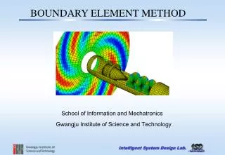
BOUNDARY ELEMENT METHOD. School of Information and Mechatronics Gwangju Institute of Science and Technology. Numerical Techniques. Finite Difference. operates directly on the governing differential equation using finite difference approximation to generate system of algebraic equations.

BOUNDARY ELEMENT METHOD
E N D
Presentation Transcript
BOUNDARY ELEMENT METHOD School of Information and Mechatronics Gwangju Institute of Science and Technology
Numerical Techniques Finite Difference operates directly on the governing differential equation using finite difference approximation to generate system of algebraic equations. Finite Element operates on the equivalent governing integral relation using piecewise ( element ) simple ( usually polynomial ) interpolations of domain node-point response quantities. Boundary Element operates on the equivalent governing integral relation using piecewise ( element ) simple ( usually polynomial ) interpolations of boundary node-point response quantities. Uses fundamental solutions ( Green’s function )
F Discretization Finite Difference Grid Finite Element Mesh For the numerical solution of a continuum problem, all three methods approximate the governing differential equation to the algebraic equation by using discretization. Boundary Element Mesh
Comparisons Advantage Disadvantage • Awkward for infinite problem • Requires very fine grids • Extremely general • No numerical integration Finite Difference • Requires domain meshes • Awkward for infinite problems • Requires integral relation from variational principle or weighted residual formulation • Integration of simple function • Usually symmetric matrices Finite Element • Usually nonsymmetrical matrices • Requires integral relation, plus transformation to boundary formulation using fundamental solution • Requires only boundary meshes • Ideal for infinite problem Boundary Element
BEM ( Boundary Element Method ) • Transform the governing differential equation into equivalent integral equation • Transform the domain integral equation into boundary integral equation • using Gauss-Green theorem, divergence theorem, or reciprocal theorem. • This last transformation involves certain known solution( fundamental solution ). • This fundamental solution generally describes the response of an infinite • medium to a point excitation.
Mathematical Preliminaries for BEM Boundary SurfaceS dS • Divergence Theorem VolumeV n Surface normal • Green’s Second Identity dV • Scalar functions : f , g • vector function : f • Betti’s Reciprocal Theorem ForcesA DisplacementsB = ForcesB DisplacementsA for any two loading conditions A and B
Potential Flow Examples. Heat transfer: Electrostatics: Groundwater Flow: Boundary SurfaceS Potentials u temperature Flux density q heat flux density Conductivity k thermal conductivity Sources b internal heat source VolumeV Potentials u voltage Flux density q current density Conductivity k electrical permittivity Sources b current source • Potentials : u • Flux density : q • Sources : b Potentials u head of water Flux density q flow rate Conductivity k permeability Sources b fluid entry and exit Laplace equation : If there are internal sources b then the equation becomes Poisson equation, . The normal flux density is with the conductivity k.
Potential Flow - Fundamental Solution Field point pf For Dirac delta source R Ry Rx ps Source point Fundamental Solution • For 2D, and • For 3D, and
Potential Flow – Derivation Multiply the fundamental solution by Laplace equation Multiply the potential by fundamental equation Subtract from Integrate equation on the volume V
Potential Flow – Boundary Integral Equation Using Green’s second Identity, equation is is a coefficient at ps . in the domain, c(ps) should be 1. if ps is located on the smooth boundary , c(ps) should be 1/2. out of the domain , c(ps) should be 0. Since , Boundary Integral Equation
Potential Flow – Boundary element 1D element 2D element 2D element 2 nodes 4 nodes 3 nodes 3 nodes 8 nodes 6 nodes
Potential Flow – Discretization Boundary Integral Equation including elements Interpolation using Shape function N, and and are the ith nodal values of potential and velocity at the boundary, respectively. The matrix form is
Linear Stress Analysis Equilibrium equation x3 C t h = perpendicular distance from O to the plane with normal n dS = area of triangle ABC dSi = area of triangle OCB ifi = 1, OCA ifi = 2, OAB ifi = 3 dV = volume of the tetrahedron = h dS / 3 ti= ithcomponent of tractions on the surface ij= ithcomponent of tractions on the surface bi = ithcomponent of a body force density Body force includes gravity, magnetic, inertia force, etc. n B O x2 A x1
Linear Stress Analysis The net resultant of forces that act on the body must be zero in a state of equilibrium. Thus, the quantification of the equilibrium statement is Using Cauchy stress transformation, , Three equilibrium equation governing the behavior of the stress component or The dynamic equilibrium becomes
Linear Stress Analysis – Reciprocal theorem Traction t* Traction t Surface S SurfaceS Volume V VolumeV Body force b Body force b* Displacement u Displacement u* Original loading condition Complementary load case Using Betti’s reciprocal theorem
Linear Stress Analysis – Choosing the complementary load case Neglect the body force b for simplicity in this derivation. 0 Case ( t, u, b ) represents the real loading but Case ( t*, u*, b* ) is completely arbitrary. By choosing Dirac delta function, we can make the equation much simpler. Boundary Integral Equation
Linear Stress Analysis – fundamental solution Displacement • For 2D, is Poisson’s ratio • is shear modulus ij is kronecker delta • For 3D, Traction • For 2D, = 1 and = 2 • For 3D, = 2 and = 3
Linear Stress Analysis – Body force The body force add a further term, making the boundary integral equation now The volume integral term in equation must be computed somehow to become part of the right hand side of the equation. Since b and u* are known, the integral can be obtained as a constant value. When fictitious source is at any one node, volume integral will be a single value. The matrix form is