Introduction

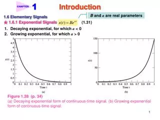
1. 1 CHAPTER Introduction B and a are real parameters 1.6 Elementary Signals ★ 1.6.1 Exponential Signals (1.31) • Decaying exponential, for which a < 0 • Growing exponential, for which a > 0 Figure 1.28 (p. 34)(a) Decaying exponential form of continuous-time signal. (b) Growing exponential form of continuous-time signal.

2. 1 CHAPTER Introduction Ex. Lossy capacitor: Fig. 1-29. KVL Eq.: (1.32) RC = Time constant (1.33) Figure 1.29 (p. 35)Lossy capacitor, with the loss represented by shunt resistance R. Discrete-time case: (1.34) where Fig. 1.30

3. 1 CHAPTER Introduction Figure 1.30 (p. 35)(a) Decaying exponential form of discrete-time signal. (b) Growing exponential form of discrete-time signal.

4. 1 CHAPTER Introduction ★ 1.6.2 Sinusoidal Signals ◆Continuous-time case: Fig. 1-31 (1.35) where periodicity

5. 1 CHAPTER Introduction Figure 1.31 (p. 36)(a) Sinusoidal signal A cos( t + Φ) with phase Φ = +/6 radians. (b) Sinusoidal signal A sin (t + Φ) with phase Φ = +/6 radians.

6. 1 CHAPTER Introduction Ex. Generation of a sinusoidal signal Fig. 1-32. Circuit Eq.: (1.36) (1.37) where Figure 1.32 (p. 37)Parallel LC circuit, assuming that the inductor L and capacitor C are both ideal. (1.38) Natural angular frequency of oscillation of the circuit ◆Discrete-time case : (1.39) Periodic condition: (1.40) or (1.41) Ex. A discrete-time sinusoidal signal: A = 1,  = 0, and N = 12. Fig. 1-33.

7. 1 CHAPTER Introduction Figure 1.33 (p. 38)Discrete-time sinusoidal signal.

8. 1 CHAPTER Introduction Example 1.7 Discrete-Time Sinusoidal Signal A pair of sinusoidal signals with a common angular frequency is defined by and • Both x1[n] and x2[n] are periodic. Find their common fundamental period. • Express the composite sinusoidal signal In the form y[n] = Acos(n + ), and evaluate the amplitude A and phase . <Sol.> (a) Angular frequency of both x1[n] and x2[n]: This can be only for m = 5, 10, 15, …, which results in N = 2, 4, 6, … (b) Trigonometric identity: Let  = 5, then compare x1[n] + x2[n] with the above equation to obtain that

9. 1 CHAPTER Introduction • =   / 6 Accordingly, we may express y[n] as

10. ★ 1.6.3 Relation Between Sinusoidal and Complex Exponential Signals 1. Euler’s identity: (1.41) (1.42) Complex exponential signal: (1.35) (1.43) ◇ Continuous-time signal in terms of sine function: (1.44) (1.45)

11. 1 CHAPTER Introduction 2. Discrete-time case: (1.46) and (1.47) 3. Two-dimensional representation of the complex exponential e j  n for  = /4 and n = 0, 1, 2, …, 7. : Fig. 1.34. Projection on real axis: cos(n); Projection on imaginary axis: sin(n) Figure 1.34 (p. 41)Complex plane, showing eight points uniformly distributed on the unit circle.

12. 1 CHAPTER Introduction ★ 1.6.4 Exponential Damped Sinusoidal Signals (1.48) Example for A = 60,  = 6, and  = 0: Fig.1.35. Figure 1.35 (p. 41)Exponentially damped sinusoidal signal Ae at sin(t), with A = 60 and  = 6.

13. 1 CHAPTER Introduction Ex. Generation of an exponential damped sinusoidal signal Fig. 1-36. Circuit Eq.: (1.49) (1.50) Figure 1.36 (p. 42)Parallel LRC, circuit, with inductor L, capacitor C, and resistor R all assumed to be ideal. where (1.51) Comparing Eq. (1.50) and (1.48), we have

14. x[n] 1 n 3 2 1 0 1 2 3 4 ◆ Discrete-time case: (1.52) ★ 1.6.5 Step Function Figure 1.37 (p. 43)Discrete-time version of step function of unit amplitude. ◆ Discrete-time case: (1.53) Fig. 1-37. ◆ Continuous-time case: (1.54) Figure 1.38 (p. 44)Continuous-time version of the unit-step function of unit amplitude.

15. 1 CHAPTER Introduction Example 1.8 Rectangular Pulse Consider the rectangular pulse x(t) shown in Fig. 1.39 (a). This pulse has an amplitude A and duration of 1 second. Express x(t) as a weighted sum of two step functions. <Sol.> 1. Rectangular pulse x(t): (1.55) (1.56)

16. 1 CHAPTER Introduction Figure 1.39 (p. 44)(a) Rectangular pulse x(t) of amplitude A and duration of 1 s, symmetric about the origin. (b) Representation of x(t) as the difference of two step functions of amplitude A, with one step function shifted to the left by ½ and the other shifted to the right by ½; the two shifted signals are denoted by x1(t) and x2(t), respectively. Note that x(t) = x1(t) – x2(t).

17. 1 CHAPTER Introduction Example 1.9 RC Circuit Find the response v(t) of RC circuit shown in Fig. 1.40 (a). <Sol.> 1. Initial value: 2. Final value: 3. Complete solution: (1.57) Figure 1.40 (p. 45)(a) Series RC circuit with a switch that is closed at time t = 0, thereby energizing the voltage source. (b) Equivalent circuit, using a step function to replace the action of the switch.

18. 1 CHAPTER (t) a(t) Figure 1.41 (p. 46)Discrete-time form of impulse. Introduction ★ 1.6.6 Impulse Function Figure 1.41 (p. 46)Discrete-time form of impulse. ◆ Discrete-time case: (1.58) Fig. 1.41 Figure 1.42 (p. 46)(a) Evolution of a rectangular pulse of unit area into an impulse of unit strength (i.e., unit impulse). (b) Graphical symbol for unit impulse. (c) Representation of an impulse of strength a that results from allowing the duration Δ of a rectangular pulse of area a to approach zero.

19. 1 CHAPTER Introduction ◆ Continuous-time case: Dirac delta function (1.59) (1.60) 1. As the duration decreases, the rectangular pulse approximates the impulse more closely. Fig. 1.42. 2. Mathematical relation between impulse and rectangular pulse function: • x(t): even function of t,  = duration. • x(t): Unit area. (1.61) Fig. 1.42 (a). 3. (t) is the derivative of u(t): 4. u(t) is the integral of (t): (1.62) (1.63)

20. 1 CHAPTER Introduction Example 1.10 RC Circuit (Continued) For the RC circuit shown in Fig. 1.43 (a), determine the current i (t) that flows through the capacitor for t 0. <Sol.> 1. Voltage across the capacitor: 2. Current flowing through capacitor:

21. 1 CHAPTER Introduction ◆ Properties of impulse function: (1.68) 1. Even function: (1.64) 2. Sifting property: Ex. RLC circuit driven by impulsive source: Fig. 1.45. (1.65) 3. Time-scaling property: For Fig. 1.45 (a), the voltage across the capacitor at time t = 0+ is (1.66) (1.69) <p.f.> Fig. 1.44 1. Rectangular pulse approximation: (1.67) 2. Unit area pulse: Fig. 1.44(a). Time scaling: Fig. 1.44(b). Area = 1/a Restoring unit area ax(at)

22. 1 CHAPTER Introduction Figure 1.44 (p. 48)Steps involved in proving the time-scaling property of the unit impulse. (a) Rectangular pulse xΔ(t) of amplitude 1/Δ and duration Δ, symmetric about the origin. (b) Pulse xΔ(t) compressed by factor a. (c) Amplitude scaling of the compressed pulse, restoring it to unit area. Figure 1.45 (p. 49)(a) Parallel LRC circuit driven by an impulsive current signal. (b) Series LRC circuit driven by an impulsive voltage signal.

23. 1 CHAPTER Introduction ★ 1.6.7 Derivatives of The Impulse Problem 1.24 1. Doublet: (1.70) 2. Fundamental property of the doublet: (1.71) (1.72) 3. Second derivative of impulse: (1.73) ★ 1.6.8 Ramp Function 1. Continuous-time case: (1.74) Fig. 1.46 or (1.75)

24. 1 CHAPTER x[n] 4 n 3 2 1 0 1 2 3 4 Introduction 2. Discrete-time case: Figure 1.46 (p. 51)Ramp function of unit slope. (1.76) or (1.77) Fig. 1.47. Figure 1.47 (p. 52)Discrete-time version of the ramp function. Example 1.11 Parallel Circuit Consider the parallel circuit of Fig. 1-48 (a) involving a dc current source I0 and an initially uncharged capacitor C. The switch across the capacitor is suddenly opened at time t = 0. Determine the current i(t) flowing through the capacitor and the voltage v(t) across it for t 0. <Sol.> 1. Capacitor current:

25. 1 CHAPTER Introduction 2. Capacitor voltage: Figure 1.48 (p. 52)(a) Parallel circuit consisting of a current source, switch, and capacitor, the capacitor is initially assumed to be uncharged, and the switch is opened at time t = 0. (b) Equivalent circuit replacing the action of opening the switch with the step function u(t).

26. 1 CHAPTER Introduction 1.7 Systems Viewed as Interconnections of Operations A system may be viewed as an interconnection of operations that transforms an input signal into an output signal with properties different from those of the input signal. 1. Continuous-time case: (1.78) 2. Discrete-time case: Figure 1.49 (p. 53)Block diagram representation of operator H for (a) continuous time and (b) discrete time. (1.79) Fig. 1-49 (a) and (b). Example 1.12 Moving-average system Consider a discrete-time system whose output signal y[n] is the average of the three most recent values of the input signal x[n], that is Formulate the operator H for this system; hence, develop a block diagram representation for it.

27. 1 CHAPTER Introduction <Sol.> 1. Discrete-time-shift operator Sk: Fig. 1.50. Shifts the input x[n] by k time units to produce an output equal to x[n  k]. Figure 1.50 (p. 54)Discrete-time-shift operator Sk, operating on the discrete-time signal x[n] to produce x[n – k]. 2. Overall operator H for the moving-average system: Fig. 1-51. Fig. 1-51 (a): cascade form; Fig. 1-51 (b): parallel form.

28. 1 CHAPTER Introduction Figure 1.51 (p. 54)Two different (but equivalent) implementations of the moving-average system: (a) cascade form of implementation and (b) parallel form of implementation.

29. 1.8 Properties of Systems ★ 1.8.1 Stability 1. A system is said to be bounded-input, bounded-output (BIBO) stable if and only if every bounded input results in a bounded output. 2. The operator H is BIBO stable if the output signal y(t) satisfies the condition (1.80) Both Mx and My represent some finite positive number whenever the input signals x(t) satisfy the condition (1.81)

30. 1 CHAPTER Introduction One famous example of an unstable system: Figure 1.52a (p. 56)Dramatic photographs showing the collapse of the Tacoma Narrows suspension bridge on November 7, 1940. (a) Photograph showing the twisting motion of the bridge’s center span just before failure. (b) A few minutes after the first piece of concrete fell, this second photograph shows a 600-ft section of the bridge breaking out of the suspension span and turning upside down as it crashed in Puget Sound, Washington. Note the car in the top right-hand corner of the photograph.(Courtesy of the Smithsonian Institution.)

31. 1 CHAPTER Introduction Example 1.13 Moving-average system (continued) Show that the moving-average system described in Example 1.12 is BIBO stable. <p.f.> 1. Assume that: 2. Input-output relation: The moving-average system is stable.

32. 1 CHAPTER Introduction Example 1.14 Unstable system Consider a discrete-time system whose input-output relation is defined by where r > 1. Show that this system is unstable. <p.f.> 1. Assume that: 2. We find that With r > 1, the multiplying factor rn diverges for increasing n. The system is unstable. ★ 1.8.2 Memory A system is said to possess memory if its output signal depends on past or future values of the input signal. A system is said to possess memoryless if its output signal depends only on the present values of the input signal.

33. 1 CHAPTER Introduction Ex.: Resistor Memoryless ! Ex.: Inductor Memory ! Ex.: Moving-average system Memory ! Ex.: A system described by the input-output relation Memoryless ! ★ 1.8.3 Causality A system is said to be causal if its present value of the output signal depends only on the present or past values of the input signal. A system is said to be noncausal if its output signal depends on one or more future values of the input signal.

34. 1 CHAPTER Introduction Ex.: Moving-average system Causal ! Ex.: Moving-average system Noncausal !  Causality is required for a systems to be capable of operating in real time. ★ 1.8.4 Invertibility A system is said to be invertible if the input of the system can be recovered from the output. Figure 1.54 (p. 59)The notion of system invertibility. The second operator Hinv is the inverse of the first operator H. Hence, the input x(t) is passed through the cascade correction of H and Hinv completely unchanged. 1. Continuous-time system: Fig. 1.54. x(t) = input; y(t) = output H = first system operator; Hinv = second system operator

35. 1 CHAPTER Introduction 2. Output of the second system: H inv = inverse operator 3. Condition for invertible system: I = identity operator (1.82) Example 1.15 Inverse of System Consider the time-shift system described by the input-output relation where the operator St0 represents a time shift of t0 seconds. Find the inverse of this system. <Sol.> 1. Inverse operator St0: 2. Invertibility condition: Time shift of t0

36. 1 CHAPTER Introduction Example 1.16 Non-Invertible System Show that a square-law system described by the input-output relation is not invertible. Since the distinct inputs x(t) and  x(t) produce the same output y(t). Accordingly, the square-law system is not invertible. <p.f.> ★ 1.8.5 Time Invariance A system is said to be time invariance if a time delay or time advance of the input signal leads to an identical time shift in the output signal.  A time-invariant system do not change with time. Figure 1.55 (p.61) The notion of time invariance. (a) Time-shift operator St0 preceding operator H. (b) Time-shift operator St0 following operator H. These two situations are equivalent, provided that H is time invariant.

37. 1 CHAPTER Introduction 1. Continuous-time system: 2. Input signal x1(t) is shifted in time by t0 seconds: St0 = operator of a time shift equal to t0 3. Output of system H: (1.83) 4. For Fig. 1-55 (b), the output of system H is y1(t t0): (1.84) 5. Condition for time-invariant system: (1.85)

38. 1 CHAPTER y1(t) = i(t) x1(t) = v(t) Introduction Example 1.17 Inductor The inductor shown in figure is described by the input-output relation: where L is the inductance. Show that the inductor so described is time invariant. <Sol.> Response y2(t) of the inductor to 1. Let x1(t) x1(t  t0) x1(t  t0) is (A) 2. Let y1(t t0) = the original output of the inductor, shifted by t0 seconds: (B) 3. Changing variables: (A) Inductor is time invariant.

39. 1 CHAPTER y1(t) = i(t) x1(t) = v(t) Introduction Example 1.18 Thermistor Let R(t) denote the resistance of the thermistor, expressed as a function of time. We may express the input-output relation of the device as Show that the thermistor so described is time variant. <Sol.> 1. Let response y2(t) of the thermistor to x1(t  t0) is 2. Let y1(tt0) = the original output of the thermistor due to x1(t), shifted by t0 seconds: 3. Since R(t)  R(t  t0) Time variant!