Download
1 / 76
760 likes | 921 Vues
Towards Resilient and Practical Geometric Routing for WSNs. Ke Liu Ph.D. Candidate Dept. of CS, Binghamton University Advisor: Nael Abu-Ghazaleh. Background and Motivation Virtual Coordinates System (VCS) Geometric Routing on VCS Contribution Anomalies in VCS: dimensional degradation

E N D
Towards Resilient and Practical Geometric Routing for WSNs Ke Liu Ph.D. Candidate Dept. of CS, Binghamton University Advisor: Nael Abu-Ghazaleh
Background and Motivation Virtual Coordinates System (VCS) Geometric Routing on VCS Contribution Anomalies in VCS: dimensional degradation Complementary Routing: HGR and SPGR AVCS: Aligned VCS AGSR: Aligned Greedy and Spanning-Path Routing Security Issues Research Agenda Conclusion Outlines
Routing for WSNs • Support the special communication pattern • Low overhead • Energy efficient • Redundancy control: data fusion • Security • Other Req: real-time, MAC aware, etc. • Traditional ones such as DSR do not fit
Geographic Routing (GPSR) • Proposed by B. Karp (MobiCom 2000), know as Greedy and Perimeter Stateless Routing (GPSR) • A similar one proposed by Hannes Frey, know as Greedy and Face routing (GFG) • Stateless: no path information, no (traditional) routing table. Only locations of neighborhood is used.
Geographic Routing Limitation • Accurate Location • GPS is expensive • Indoor application • Localization Algorithm is not Accurate: 40% localization error is common • Perimeter Routing is not efficient • (Possible hundred) times longer than greedy forward. • Fail facing Localization error
Virtual Coordinates System (VCS) • Reference (anchor) nodes are served as bases of VCS • Each node sets up its VC as hop counts to reference nodes • As localization algorithm at first, later independently used, replacing the physical coordinate system (GeoCS or PCS) • Only based on communication connectivity • Physical voids are avoided -- mostly • Virtual voids arise, NOT with physical voids
It is possible Dis(A, B) == Dis(A, C) Packet arrives at A can not be forwarded to C, since B is as far as A to C Even there is a path from A to C through B, forwarding would fail VCS Anomaly: Forwarding Void
Important Definitions • Given a graph G(V, E) • Component: C(V’,E’), |V’| >= 2 • Node cutVc: |Vc| >=2, and {Vc == V’, or removing Vc would disconnect the rest of C(V’, E’) from G(V, E)} • Network connectivity: the minimal size of any component • Determinant Component: some anchor node in Vc • Indeterminate Component • Uniqueness DegreeUd: number of all unique virtual coordinate values for all nodes in network
Dimensional Degradation: Dd • Maximal number of virtual dimensions (virtual anchors) which can increase the naming uniqueness (Ud) • if the Ud of a n-dimensional virtual coordinatesystem on a network is x, and the Ud of a (n+1)-dimensionalvirtual coordinate system is also x, we say the Dd of this network is n.
Theorem 1: The Dd of a 1-connected graph is 1 • A node cut Vc contains only this node, separate the network into 2 parts, one is determinant component, another is indeterminate component • Increasing the virtual dimension means select one more node in the determinant component as new anchor • Values for the new virtual dimension do not increase the naming uniqueness
Theorem 3 • If using the current VCS set up procedure, then complete graph suffers most • It convergences to shortest path routing.
Quantization Error • Virtual coordinate values are integers – hop-count based • Nodes at different distances to some anchor node, receive the same value on the corresponding virtual dimension • For each hop, a noise about ½ Radio Range can be introduced. As nodes getting farther to the anchor, noise increase tremendously
Anchor Placement Anomaly • Connection to Dimensional Degradation is not clear • Anchors at center decrease the dimensional degradation of the network
Backtracking for GR on VCS • Virtual Anomalies do not arise as the physical void for the same reason • Observation: virtual anomalies do not happen at the same place as physical void (mostly or absolutely?) • Heuristics: to combine the VCS as PCS for geometric routing (complementary phase)
HGR: hybrid geometric routing • When greedy forwarding in geographic routing fails, greedy forwarding is continued on VCS. • When greedy forwarding fails on VCS, HGR works based on knowing PCS and VCS, as complementary routing • Axis by Axis basis • In current axis • Packet is forwarded to node closer to sink (physical distance) among nodes with the same VC • When void reached, reverse the backtracking direction or skip to next axis • When all axis are tried, HGR fails (possibly)
Spanning-Path VCS and Routing • Why not use ONLY VCS – no localization at all • Our intuition was “impossible” in the proposal – • Yes, it is impossible if using the same VCS setting up • No, it is possible if we think it again • Current VCS setting up breaks the naming uniqueness of coordinate system, we pick it up here • Giving each node a unique ID (VC value) globally and dynamically
Related Work • Blind Searching: VCap, LCR • VCap: Random detour • LCR: each node records each packet forwarded • Data Flooding: BVR • Send the packet to the closest anchor node • Anchor node scope floods the packet • VCS Upgrading: GSpring • Elect one more node as a new anchor
Motivation: Spanning-Tree • GEM: Using spanning-tree structure (VPCS), as localization alogrithm • GDSTR: • Spanning-Tree structure: Hull Tree • Convex Hull: aggregate all descendent nodes as a convex hull – a polygon covers the area of descendent nodes • Negative false: failed to confirm some node in convex hull – routing failure • Although those Spanning-tree structure based solution fail, we still believe it is a solution
Spanning-Path VCS • One node is elected as anchor node • DFS algorithm to set up a spanning-tree structure • Each node is assigned a unique ID (SPVC) • Maximal Range: After all descendent nodes are assigned SPVCs, the maximal SPVC is assigned to the root as its max range
Spanning-Path Geometric Routing • Descendent Range: node’s SPVC node’s max range • Forwarding candidates: any node whose descendent range contains the destination’s SPVC • Using the one with the smallest descendent range as next hop
SPGR Optimization: BFS based • SPGR: DFS • SPGR: BFS
SPGR Optimization: Multiple Anchors • Multiple anchors are selected: 4 corners, and one in the middle (center or random) • Similar as BVR: • On one of virtual dimensions, the source and destination is closest (difference between their SPVC values) • Using this dimension as the routing base • Do not change virtual dimension during the routing • It is not a “Real” optimization, just an experiment • Simulation shows trivial improvement • Demanding future work
SPGR Evaluation: Path Stretch • Perimeter routing suffers more, when density increases • SPGR benefit • BFS optimization improve, as intuition • Multiple anchor improve slightly
SPGR Evaluation: Anchor placement • Corner anchor leads to longer path – more unbalanced spanning-tree structure • Center anchor – more balanced tree structure • Random anchor in between
SPGR Evaluation: Anchor Load • Corner anchor, lower load, since unbalanced tree leads to less path go through root • Center anchor: higher load by balanced tree • So using corner anchor or center anchor, is a trade-off
Aligned VCS (AVCS): Intuition • Quantization Error: higher effect with higher density • VCS is set up based only on communication connectivity, but not all connectivity information was used for VCS • Greedy Forwarding is used less with VCS than with PCS, leading to much more use of inefficient complementary routing (backtracking)
AVCS: Alignment • For Node A and all its Neighbors (N) in VCS, we have • The alignment function is used in AVCS as The alignment is the average of virtual coordinates of the given node’s neighborhood.