Cubic Spline Interpolants
Learn about cubic spline interpolants, their properties and boundary conditions for accurate function approximations.

Cubic Spline Interpolants
E N D
Presentation Transcript
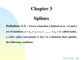
Chapter 3 Splines Definition (3.1) : Given a function f defined on [a , b] and a set of numbers, a = x0 < x1 < x2 < ……. < xn = b, called nodes, a cubic spline interpolantS, for f is a function that satisfies the following condition:
(3.1). S is a cubic polynomial, denoted Sj, on the subinterval [ xj , xj + 1] for each j = 0, 1, ..., n-1. (3.2). S(xj) = f(xj) for each j = 0, 1, …, n. (The spline passes through each data point.)
(3.3). Sj + 1 (xj + 1 ) = Sj (xj + 1) for each j = 0, 1, …, n-2. ( The spline forms a continuous function.) (3.4). S¢j + 1(xj + 1) = S¢j (xj + 1) for each j = 0, 1, …, n-2. ( The spline forms a smooth function.) (3.5). S¢¢j + 1(xj + 1) = S¢¢j (xj + 1) for each j = 0, 1, …, n-2. ( The second derivative is continuous.)
(3.6). One of the following set of boundary conditions is satisfied: (4.6.1) S¢¢(x0) = S¢¢(xn) = 0 ( free or natural boundary) (4.6.2) S¢(x0) = f ¢(x0) and S¢(xn) = f ¢(xn) ( Clamped boundary) Although cubic splines are defined with other boundary conditions, the conditions given above are sufficient for our purposes. When the free boundary conditions occur, the spline is called a natural cubic spline.
and its graph approximates the shape, which a long flexible rod would assume if forced to go through each of the data points {( x0 , f(x0)) , ( x1 , f(x1)) , …, ( xn , f(xn))}. Similarly, when the clamped boundary conditions occur, the spline is called a clamped cubic spline. In general, clamped boundary conditions lead to more accurate approximations since they include more information about the function.
However, for this type of boundary conditions to hold, it is necessary to have either the value of the derivative at the endpoints or acceptable approximations to those values. Hence we concentrate here only on natural cubic interpolants. To construct the cubic spline interpolant for a given function f, the conditions in the definition (3.1) are applied to the cubic polynomials.
Sj(x) = aj + bj (x – xj) + cj (x – xj)2 + dj (x – xj )3; for each j = 0, 1, …, n-1. Clearly, Sj(xj) = aj = f(xj), and if conditions (3.3) are applied, aj + 1 = Sj + 1(xj + 1) = Sj (xj + 1) = aj + bj (xj +1 – xj) + cj (xj + 1 – xj)2 + dj (xj + 1 – xj )3 for each j = 0, 1, …, n-2.
Since the term (xj+1 – xj) will be used repeatedly in this development, it is convenient to introduce the notation hj = xj+1 – xj ; for each j = 0, 1, …, n-1. If we also define an = f(xn), then the equation aj + 1 = aj + bjhj + cjhj2 + djhj3; holds for each j = 0 , 1, …, n-1. (3.9) In a similar manner, define bn = S¢(xn) and observe that Sj¢(x) = bj + 2cj( x – xj) + 3dj (x- xj)2 Implies Sj¢(xj) = bjfor each j = 0, 1, …, n-1.
Appling condition (3.4), we get bj + 1 = bj + 2cjhj + 3djhj2 ; for each j = 0, 1, …, n-1. (3.10) Another relationship between the coefficients of Sj is obtained by defining cn = S¢¢(xn) /2 and applying condition (3.5). In this case, cj + 1 = cj + 3djhj; for each j = 0, 1, …, n-1. (3.11) Solving for dj in Eq. (3.11) and substituting this value into Eqs. (3.9) and (3.10) gives the new equations
aj + 1 = aj + bjhj + (hj2 / 3) (2cj + cj+ 1 ) ; for each j = 0, 1, …, n-1. (3.12) and bj + 1 = bj + hj (cj + cj + 1) ; for each j = 0, 1, …, n-1. (3.13) The final relationship involving the coefficients is obtained by solving the appropriate equation in the form of equation (3.12), first for bj, bj = (1/hj) (aj +1 – aj) – (hj / 3) (2cj + cj +1) (3.14) and then, with a reduction of the index, for bj – 1, bj –1 = (1 / hj – 1) (aj – aj –1) – (hj –1 / 3)(2cj –1 + cj ).
Substituting these values into the equation derived from Eq. (3.13), when the index is reduced by 1, gives the linear system of equations hj –1 cj – 1+ 2(hj – 1 + hj )cj+hjcj +1 = (3/hj)(aj +1 – aj) – (3/ hj – 1)(aj – aj –1 ); for each j = 0, 1, …, n-1. (3.15) This system involves, only cj¢ s as unknowns, since the value of hj¢sand aj¢s are given by the spacing of the nodes xj¢ s and the value of f at the nodes.
Note that once the value of cj¢ s are known, it is a simpler matter to find the remainder of the constants bj ¢s from Eq. (3.14) and dj¢ s from Eq. (3.11) and to construct the cubic polynomials Sj¢ s. The natural boundary conditions in this case imply that cn = S¢¢(xn) / 2 = 0that 0 =S¢¢(x0) = 2c0 +6d0(x0 – x0) So, c0 = 0.
The two equations c0 = 0and cn = 0together with the equations in (3.15) produce a linear system described by the vector equation Ax = b, where A is ( n+1 )*( n +1) matrix given below. A =
With x = and b =
Go to Chapter 4 Note : Solution of this system is usually obtained using Crouts Algorithm. End of Chapter 3