Download
1 / 16
160 likes | 277 Vues
This study explores the role of temperature-dependent rheology in hydrofracture models, particularly in the context of subduction zones. It emphasizes the interactions between water and dry peridotite and how these processes influence magmatic activity and hydration dynamics beneath tectonic plates. The research utilizes numerical simulations to analyze different scenarios, such as cold and hot slabs, and examines the transport of water in these environments. Insights from this model could advance our understanding of the physical and chemical processes governing subduction.

E N D
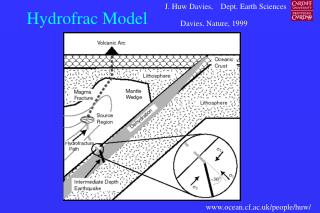
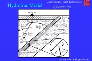
Davies, Nature, 1999 Hydrofrac Model
Temperature dependent rheology Model with temperature dependent rheology, example here would ‘eat’ all the way to the surface. Possible to get freezing out –see Kincaid and Sacks. We know we get magmas therefore I prefer hot end-point => need means to stop eating all the way to surface. Possibly lithosphere in wedge corner is crust (i.e. buyoancy not rheology keeps things near surface) Starting Model Model a little time later – not steady-state
Water reacts with mantle – Davies (1994) Davies and Stevenson (1992) Water reacts with largely dry peridotite Path of water in hydrated mineral melting Water enters wedge Water flow as free phase Mantle largely dry Flow of mantle
My Favourite Model (Iwamori, EPSL,1998) Equilibrium, 130Ma, 6cm/yr Equilibrium, 10Ma, 6cm/yr
Iwamori (EPSL, 1998) Disequilibrium, 130Ma, 6cm/yr
Iwamori (EPSL, 1998 – Fig Cap for Fig 5) • Fig. 5. Distribution of H2O (left) and melt (right). (a) For a relatively cold slab (age 130 Myr) with a constant subduction velocity, of ~6 cm/year. A cross-sectional area of 250x250 km region with a fixed crust of 30 km thick is divided into a regular grid for numerical calculations, with a finer triangular grid at the slab¯wedge interface and at the bottom of the slab for preventing artificial diffusion of H2O. The thickness of rigid slab can be defined as 2.32 (kt)1/2 where k is the thermal diffusivity. If k = 10-6 m2 s-1, then thickness = 150km. In both the oceanic side (lower left corner) and the mantle wedge side (upper right) of the rigid slab, the solid flow is assumed to be described by analytic corner flow solutions of incompressible fluid with constant viscosity. The dotted lines in the mantle wedge indicate the stream lines. The thermal boundary conditions are as follows: a surface temperature of 273 K; an error function gradient for the plate age of 130 Myr and an adiabatic gradient underneath for the oceanic side boundary; a linear gradient within the crust and within a thermal boundary layer of 12 km beneath the crust to produce the surface heat flux of 0.115 W/m2, and an adiabatic gradient underneath the arc side boundary, which gives the potential temperature ~1250°C; zero heat flux at the bottom boundary.The solid lines indicate the isothermal contours with a 200K interval. A steady geothermal structure for H2O-free subduction of the slab was assumed for an initial condition where no melt exists, then the slab with 6 wt% H2O started to subduct. The elapsed time for this snapshot is 7.1 Myr. (b) For a hot slab (age of 10 Myr) with a constant subduction velocity of ~6 cm/year. The thickness of rigid slab is 40km. The other conditions are the same as in (a). The elapsed time for this snapshot is 4.1 Myr. (c) For a case involving disequilibrium transportation of H2O. A small portion of the aqueous fluid (8% of the aqueous fluid present in each local system) is assumed to be isolated chemically in the local system. Consequently, once the aqueous fluid is produced, it can survive and continue to migrate even if the surrounding solid and melt are not saturated with H2O. The other conditions are the same as in (a). The elapsed time for this snapshot is 2.9 Myr.
Physical and Chemical Constraints on SZ processes • Physical – (Many subduction zones – many experiments) • Plate velocities, Age of subducting lithosphere, thickness overriding plate crust • Shape of Benioff zone, double zone? Dip? • Location of magmatism – See below. Rate of magmatism, temp. of lavas • Surface shape – trench depth, outer arc rise – GPS, satellite • Heat flux – Broad scale good, but at local scale there are many poorly understood processes • Seismology, • Tomography – Velocity (P,S), Attenuation, low vel. zone (crust?) • Anisotropy – interpretation – water? • Focal mechanisms, stress regimes • 3D seismic – ANCORP, Shipley et al., Banks et al., • Down- and up-dip extent of mega-thrust plane • Lab measurements – rheology, anisotropy, dihedral angle • Electrical conductivity • Gravity and geoid – low density/low viscosity
Chemistry – help! • Inputs – Drilling of ocean sediments and basalts • Outputs – Composition • Major elements – differentiation, primary magmas eq. temp, degree of melting • Trace elements – LILE/HFSE, B, degree of melting • Xenoliths • Isotopes - Stable/Radiogenic – Be10, U versus Pb, Th versus Be • Fluid/Melt Inclusions – water contents • Uranium decay chain isotopes – time scales – fast • Volatiles - fluxes • Expts. – Melting expts. – • Sediments, Peridotite, Basalt +/- water, composition – diamond aggregates • Partitioning – including improved theory • Thermodynamic databases – MELTS – extend to hydrous systems • Outputs from other parts of the mantle; e.g. OIB - recycled SZ plates?
Location of arc relative to Benioff zone – h Volcanic Front o.c. slab h mantle earthquakes
65 80 105 85 105 120 135 110 120 125 115 105 105 105 h (km) – constant along arc segments, but different from segment to segment – England, Engdahl et al. (unpublished)
Subduction Tomography – Zhao + Hasegawa (1993) Non-unique but a 3D constraint Resolution? Combine with 3D reflection seismics?
Temperature of Primary Magmas • Tatsumi et al., Nye and Reid, etc. • Questions – • Is this how magmas form? i.e. equilibrium, batch • Do we sample and can we identify primary magmas? Tatsumi et al., 1983 High Alumina Basalt + 1.5% water l Temperature opx+l 1320oC ol+l opx+cpx+l ol+cpx+l ol+opx+cpx+l 50km Pressure/Depth
Chemical correlations • Stolper and Newman – Water and Chemistry • Plank and Langmuir – Sediment input and volcanic output • Elliott et al. - • Etc
Melting of sediments • Claims that sediments do melt • Experiments constrain temperature of sediment melting • Therefore constraint on temperature at sediment – wedge boundary • Temperatures are generally higher than predicted by numerical thermal models (but models, while precise are not very accurate – equally interpretation of presence of melt is debatable – remember difference between fluid with high silica content and melt with high fluid contents might be small)
Constraints – Huw Stops (You start) • h – geometry • Seismic tomography • Sediment melting • Chemical correlations – including timescales • Temperature of primary magmas