Introduction to Generalized Linear Models: A Practical Approach
Learn the basics of linear and generalized linear models with simple applications and common software examples. Understand regression analysis, diagnostic tools, and handling non-linear relationships. Find out how to use multivariable regression and manage multicollinearity. Discover stepwise regression methods and degrees of freedom in regression analysis.

Introduction to Generalized Linear Models: A Practical Approach
E N D
Presentation Transcript
Introduction to Generalized Linear Models Prepared by Louise Francis Francis Analytics and Actuarial Data Mining, Inc. www.data-mines.com September 18, 2005
Objectives • Gentle introduction to Linear Models and Generalized Linear Models • Illustrate some simple applications • Show examples in commonly available software • Address some practical issues
A Brief Introduction to Regression • Fits line that minimizes squared deviation between actual and fitted values
Excel Does Regression • Install Data Analysis Tool Pak (Add In) that comes wit Excel • Click Tools, Data Analysis, Regression
Goodness of Fit Statistics • R2: (SS Regression/SS Total) • percentage of variance explained • F statistic: (MS Regression/MS Residual) • significance of regression • T statistics: Uses SE of coefficient to determine if it is significant • significance of coefficients • It is customary to drop variable if coefficient not significant • Note SS = Sum squared errors
Other Diagnostics: Residual Plot • Points should scatter randomly around zero • If not, a straight line probably is not be appropriate
Other Diagnostics: Normal Plot • Plot should be a straight line • Otherwise residuals not from normal distribution
Non-Linear Relationships • The model fit was of the form: • Severity = a + b*Year • A more common trend model is: • SeverityYear=SeverityYear0*(1+t)(Year-Year0) • T is the trend rate • This is an exponential trend model • Cannot fit it with a line
Exponential Trend – Cont. • R2 declines and Residuals indicate poor fit
A More Complex Model • Use more than one variable in model (Econometric Model) • In this case we use a medical cost index, the consumer price index and employment data (number employed, unemployment rate, change in number employed, change in UEP rate to predict workers compensation severity
One Approach: Regression With All Variables • Many variables not significant • Over-parameterization issue • How get best fitting most parsimonious model?
Stepwise Regression • Partial correlation • Correlation of dependent variable with predictor after all other variables are in model • F – contribution • Amount of change in F-statistic when variable is added to model
Stepwise regression-kinds • Forward stepwise • Start with best one variable regression and add • Backward stepwise • Start with full regression and delete variables • Exhaustive
Econometric Model Assessment • Standardized residuals more evenly spread around the zero line • R2 is .91 vs .52 of simple trend regression
Multicollinearity • Predictor variables are assumed uncorrelated • Assess with correlation matrix
Remedies for Multicollinearity • Drop one or more of the highly correlated variables • Use Factor analysis or Principle components to produce a new variable which is a weighted average of the correlated variables • Use stepwise regression to select variables to include
Degrees of Freedom • Related to number of observations • One rule of thumb: subtract the number of parameters estimated from the number of observations • The greater the number of parameters estimated, the lower the number of degrees of freedom
Degrees of Freedom • “Degrees of freedom for a particular sum of squares is the smallest number of terms we need to know in order to find the remaining terms and thereby compute the sum” • Iverson and Norpoth, Analysis of Variance • We want to keep the df as large as possible to avoid overfitting • This concept becomes particularly important with complex data mining models
Regression Output cont. • Standardized residuals more evenly spread around the zero line – but pattern still present • R2 is .84 vs .52 of simple trend regression • We might want other variables in model (i.e, unemployment rate), but at some point overfitting becomes a problem
Tail Development Factors: Another Regression Application • Typically involve non-linear functions: • Inverse Power Curve: • Hoerel Curve: • Probability distribution such as Gamma, Lognormal
Non-Linear Regression • Use it to fit a non-linear function where transformation to linear model will not work • Example • LDF = (Cumulative % Incurred at t+1)/ (Cumulative % Incurred a t) Assume gamma cumulative distribution
Example: Inverse Power Curve • Can use transformation of variables to fit simplified model: LDF=1+k/ta • ln(LDF-1) =a+b*ln(1/t) • Use nonlinear regression to solve for a and c • Uses numerical algorithms, such as gradient descent to solve for parameters. • Most statistics packages let you do this
Nonlinear Regression: Grid Search Method • Try out a number of different values for parameters and pick the ones which minimize a goodness of fit statistic • You can use the Data Table capability of Excel to do this • Use regression functions linest and intercept to get k and a • Try out different values for c until you find the best one
Claim Count Triangle Model • Chain ladder is common approach
Claim Count Development • Another approach: additive model • This model is the same as a one factor ANOVA
ANOVA: Two Groups • With only two groups we test the significance of the difference between their means • Many years ago in a statistics course we learned how to use a t-test for this
Regression With Dummy Variables • Let Devage24=1 if development age = 24 months, 0 otherwise • Let Devage36=1 if development age = 36 months, 0 otherwise • Need one less dummy variable than number of ages
Apply Logarithmic Transformation • It is reasonable to believe that variance is proportional to expected value • Claims can only have positive values • If we log the claim values, can’t get a negative • Regress log(Claims+.001) on dummy variables or do ANOVA on logged data
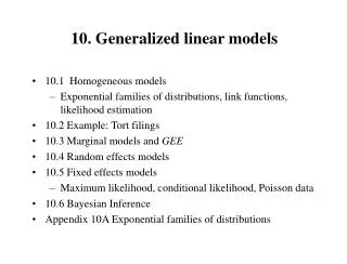
Poisson Regression • Log Regression assumption: errors on log scale are from normal distribution. • But these are claims – Poisson assumption might be reasonable • Poisson and Normal from more general class of distributions: exponential family of distributions
Specific Members of the Exponential Family • Normal (Gaussian) • Poisson • Binomial • Negative Binomial • Gamma • Inverse Gaussian