Download
1 / 30
420 likes | 1.05k Vues
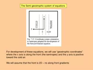
The Semi-geostrophic system of equations. For development of these equations, we will use “geostrophic coordinates” where the x axis is along the front (the isentropes) and the y axis is positive toward the cold air. We will assume that the front is 2D – no along front gradients.

E N D
The Semi-geostrophic system of equations For development of these equations, we will use “geostrophic coordinates” where the x axis is along the front (the isentropes) and the y axis is positive toward the cold air. We will assume that the front is 2D – no along front gradients
The geostrophic wind relationships are given by The hydrostatic relationship is given by where And the thermal wind relationships are given by
The equation of motion in the along front direction Where Ug and u are the along front geostrophic and ageostrophic wind components And the along front geopotential height gradient is zero because of the 2-D assumption We will now make the “geostrophic momentum approximation” Assume that there is no systematic change in the along-front ageostrophic wind The equation of motion in the along front direction becomes
Expand the total derivative: The thermodynamic equation: Since the along front flow is assumed to be in geostrophic balance we will ignore the crossed out terms
We will now introduce the absolute geostrophic momentum Note that M is conserved:
A B Take of A and add it to of B
Now consider the continuity equation Define a streamfunction for the ageostrophic flow in the y direction Substitute into the equation below to get Where: is the geostrophic forcing function
This equation is called the “Sawyer-Eliassen circulation equation” derived in papers by Sawyer (1955) and Eliassen (1962) It has the form: Which has a solution that depends on the sign of the discriminant Elliptic Parabolic Hyperbolic
We therefore require Elliptic solutions to the equation are those in which u is uniquely determined from the forcing G Use thermal wind relationship This is the QG potential vorticity! The Sawyer-Eliassen equation will have solutions provided that the air is statically stable and inertially stable, that is, the QG potential vorticity is positive. If QG Potential Vorticity is negative, solutions are non-unique because of the release of the instability.
Static stability Baroclinicity (thermal wind) Inertial stability Geostrophic deformation Diabatic heating Right side of equation represent the forcing (known from measurements or in model solution) , the streamfunction, is the response Solutions for can be obtained provided lateral and top/bottom boundary conditions are specified and the potential vorticity is positive in the domain (air is inertially, convectively and symmetrically [slantwise] stable).
Nature of the solution of the Sawyer-Eliassen Equation: A direct circulation (warm air rising and cold air sinking) will result with positive forcing. An indirect circulation (warm air sinking and cold air rising) will result with negative forcing. Isentrope Warm air Cold air Isentrope Warm air Cold air
Dynamics of frontogenesis A conceptual model of the ageostrophic circulation caused by frontogenesis On the figure on the left, Dashed lines: potential temperature Blue lines: pressure surfaces (exaggerated) Shading: isotachs (blue into screen, red out) 1. Initial condition Geostrophically-balanced weak front 2. Impulsively intensify front Stronger temperature gradient leads to more steeply sloped pressure surfaces and an increase in the pressure gradient force at both high and low levels
Dynamics of frontogenesis A conceptual model of the ageostrophic circulation caused by frontogenesis 2. Impulsively intensify front Stronger temperature gradient leads to more steeply sloped pressure surfaces and an increase in the pressure gradient force at both high and low levels 3. Air accelerates Air rises on warm side Air descends on cold side Air accelerates along isentropes toward cold air and into screen aloft Air accelerates toward warm air and out of screen in low levels
Dynamics of frontogenesis A conceptual model of the ageostrophic circulation caused by frontogenesis 3. Air accelerates Air rises on warm side Air descends on cold side Air accelerates toward cold air and into screen aloft Air accelerates toward warm air and out of screen in low levels 4. Balance is restored - Air rises and cools on warm side - Air sinks and warms on cold side - counteracts effects of frontogenesis Air cools at moist Adiabatic lapse rate • Wind speed in upper jet increases • (into screen) • Wind speed in lower jet increases • (out of screen) • - Coriolis force increases • - Geostrophic balance restored Air warms at dry Adiabatic lapse rate
The circulation describe in the last few slides can be seen clearly on the front illustrated on the cross section below
An example of a solution to the SE Equation (left) along cross section AA’ in the cyclone illustrated on the right (from Han et al. 2007). Note the circulation along the front (dashed lines are potential temperature) and within the trowal region (heavy dashed line) with sinking motion in the dry air to the south of the trowal.
An analysis of the SE forcing term Let’s rewrite using the thermal wind relationships Geostrophic shearing deformation Geostrophic stretching deformation We will examine each of these terms in isolation
Using the expression for the non-divergence of the geostrophic wind This expression can be written: Consider a jetstreak where =0 In the entrance quadrant ug increases with x while decreases with y. DIRECT CIRCULATION In the exit quadrant ug decreases with x while decreases with y. INDIRECT CIRCULATION
Consider a shear zone along a temperature gradient where =0 ug decreases with y while increases with x. INDIRECT CIRCULATION Cold advection pattern corresponds to an indirect circulation Correspondingly: Warm advection pattern corresponds to an direct circulation
Example of solution of the Sawyer-Eliassen equation The circulation about an ideal frontal zone characterized by Confluence (top) Shear (bottom) Streamlines of ageostrophic circulation (thick solid lines) Isotachs of ug (denoted U) (dashed lines) Isotachs fo vg (denoted V) (thin solid lines)
Note in this figure that both and are positive, implying frontogenesis and a direct circulation in which warm air is rising and cold air sinking. A second example: Geostrophic shearing deformation confluent flow along front
Geostrophic stretching deformation Entrance region of jet Note in this figure that both and are negative, implying frontogenesis and a direct circulation in which warm air is rising and cold air sinking.
Upper level fronts and frontogenesis • The essential mechanism for formation of upper level fronts • An indirect circulation tilts the isentropes associated with the stable stratospheric air and vortex tubes associated with vertical shear into the vertical creating: • A strong thermal gradient • Enhanced vertical vorticity • A region of high static stabilty • THE ESSENTIAL DYNAMICAL • CHARACTERISTICS OF A FRONT
Also High Ozone Measurements of Potential Vorticity and Strontium 90 in 1963 across an upper level front
Potential Vorticity Pot. Temp and wind speed Cyclonic Shear Boundary Tropopause And fronts Extremely high resolution measurements of upper level frontal structure made with a research aircraft supplemented by sondes (Shapiro 1981) Absolute Angular Momentum Absolute Angular Momentum/Pot Temp
Upper level frontogenesis Consider first a jetstreak: Shearing deformation forces frontolytic vertical circulation in exit region leading to tilting of the isentropes in a manner that supports upper level frontogenesis!
Consider next the shearing term Cold advection in the presence of cyclonic shear produces an indirect circulation leading to descending motion in warm air and ascending motion in cold air which tilts the isentropes, leading to upper level frontogenesis!
anticyclonic shear cold advection cyclonic shear cold advection direct indirect anticyclonic shear warm advection cyclonic shear warm advection direct indirect
Effect of temperature advection on the Vertical circulation about a straight jetstreak Straight jetstreak: no temperature advection Straight jetstreak: cold advection THIS PATTERN WILL CAUSE DOWNWARD MOTION ALONG JET AXIS, LEADING TO RAPID UPPER LEVEL FRONTOGENESIS Straight jetstreak: warm advection
Evolution of 500 mb heights, temperature and absolute vorticity over a 48 hr period (12 hour time intervals) As a jetstreak propagates down the back side of trough in region of cold advection, look at the rapid change in vorticity in the last 24 hours Cyclonic vorticity created by upper level frontogenesis!