Introduction to Management Science Course - Uncertainty and Decision-Making
Learn how Management Science utilizes computer technology for optimal decision-making. Explore uncertainty, choice, modelling methodologies, and more. Enhance your understanding through hands-on experience.


Introduction to Management Science Course - Uncertainty and Decision-Making
E N D
Presentation Transcript
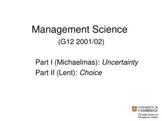
Management Science (G12 2001/02) Part I (Michaelmas): Uncertainty Part II (Lent): Choice
Today’s plan • What is Management Science and what’s the purpose of this course? • Spreadsheets as a modelling platform • Introduction to Monte Carlo Simulation • How can a computer roll a die?
Management Science • … uses computer technology to help managers make good decisions and optimise organisational processes • Operations Research and Decision Science are other names • Professional bodies • International: Institute for Operations Research and the Management Sciences (INFORMS) (www.informs.org) • UK: Operational Research Society (www.orsoc.org.uk)
Core issues of Management Science • Problem areas • decision making • Organisational process design and control • Core issues • complexity • uncertainty • choice (optimality) • Methodology: • Modelling (graphical, computer, or mathematical models)
Some important side issues • Models as communication devices • Presentation of quantitative information • Quantitative (“hard”) versus qualitative (“soft”) modelling • The “human factor” • Management information systems • Availability and reliability of data
Aim of the course • Make you aware of the potential (and limitations) of the Management Science approach • Provide you with some hands-on experience in modelling (coursework) • Discuss theoretical underpinning of some important modelling templates (exam)
Michaelmas term: Uncertainty • Computer models of uncertainty • Monte Carlo simulation • Mathematical models of uncertainty • Probability theory and stochastic processes • Modelling templates • Queuing systems • Markov chains • Others as time permits • Analysing dependencies between uncertainties • Linear regression • Forecasting the future
Supervisions and coursework • Supervision 1: Simulation in spreadsheets • Supervision 2: Stochastic processes • Supervision 3: Regression and forecasting • Coursework: Analysis of a business case using spreadsheet simulations (more later…)
Today’s plan • What is Management Science and what’s the purpose of this course? • Spreadsheets as a modelling platform • Introduction to Monte Carlo Simulation • How can a computer roll a die?
A spreadsheet is a tool that allows you to store and present quantitative information process quantitative information perform what-if analyses do much more… Spreadsheets have many disadvantages Limited data structure (2-dimensional array) Difficult to validate and document Inflexible Unreliable numerical routines Why spreadsheets?
Background Information • I assume that you are familiar with basic spreadsheet programming • If not, go through a free tutorial on the web, e.g. • http://www.compusmart.ab.ca/alummis/excel/exceltutorial.html • http://www.usd.edu/trio/tut/excel/ • http://www.jcu.edu/infoservice/training/excel/start.htm • More advanced material can be found in B.V. Liengme, A guide to Microsoft Excel for scientists and engineers (CUED Lib.)
A tip for spreadsheet modelling • Clearly separate • Data (input to the model that is not under your control) • Design parameters (input that is under your control) • The actual model (logical description of the model) • Model output ( basis for decision, often includes graphical elements) • For larger models use separate worksheets • Ideally, no cell in the logical model section contains a number • These cells only contain formulas and references to other cells, e.g. in the data or parameter section
The five stages of computer modelling (Donald Knuth) 1. Decide what you want the model to do 2. Decide how to build the model 3. Build the model 4. Debug the model 5. Trash stages 1 to 4 and start again, now that you know what you really wanted in the first place
Don’t get frustrated: A modelling process is a learning process The main benefit of building a (computer) model to analyse a problem is not the quantitative information obtained as output of the model but the enhanced understanding of the problem gained during the modelling process
Today’s plan • What is Management Science and what’s the purpose of this course? • Spreadsheets as a modelling platform • Introduction to Monte Carlo Simulation • How can a computer roll a die?
Example: A product launch • Main criterion: profitability Profit = sales*(unit price- unit costs)-fixed costs • Suppose fixed costs known • Price is a decision variable and influences sales • Pricing decision depends, among other things, on the level of competition and the reaction of the competitors to the launch (uncertain) • Unit cost is uncertain and depends on prices for raw materials, energy, etc. • Let’s look at a spreadsheet model…
The Flaw of the Average • Plugging average values into uncertain cells can lead you astray • The resulting bottom line (e.g. profit) is often not the average profit • Mathematical Reason: E(f(X))=f(E(X)) for a random variable X holds ONLY if f is linear
What do we want to achieve with a simulation model? • A single number, e.g. an average, gives very little information if model input is uncertain • Manual what-if analysis is cumbersome and biased • We want to estimate the distribution of output cells • Give a graphical representation of this distribution • cumulative distribution function • histogram
Example: Value at risk • Given a distribution function for profit, we can read off the loss x such that there is an α% chance that the loss is at least £ x • That number is called the α% value at risk (α% VAR)
10% VAR is roughly £500,000 5% VAR is roughly £800,000
Main steps of a simulation project • Understand the problem • Programme and validate a deterministic model • Determine the distribution of the uncertain inputs • Collect relevant data • Run the simulation experiments • Analyse the model output • Communicate the model and its output
Building the model… • Essential questions before you model: • What are the questions that the model is to address? • What are the interesting outputs / performance measures? • What is the appropriate level of detail? • Discuss these questions with all stakeholders in the decision situation / process • Validate the logic of your model before you enter uncertainty
Incorporating uncertainty • Estimate a probability distribution on the basis of “hard” data whenever possible • Re-sampling from historic data (see product launch example) is a simple and valid way of generating numbers for uncertain cells • Sometimes you need subjective probabilities • Get estimates from many independent experts (Delphi method) • Check sensitivity of outputs w.r.t. changing probabilities • A triangular distribution is often a good starting point • Defined by lowest, highest and most likely value
Running a simulation • Important Rule: do more replications than you expect necessary • at least several hundred • Check that running averages of outputs have settled in a steady state • E.g. record after each replication the average profit over all past replications • Do several runs and compare the results
Analysing the output • Use visual aids (histograms, distribution functions, scatter diagrams, etc.) • Use statistics (confidence intervals, hypothesis tests) • What are the implications of the results • for your model world? • for the real world?
Communicating the model and the results • IMPORTANT: Communicate regularly with all stakeholders in the decision situation or process you are modelling • Build credibility for your model • Model becomes a “language” • Forces you to be as simple as possible • Forces you to be as relevant as possible
A word about simulation platforms • Spreadsheets are useful for the simulation of many day-to-day decision problems • They are NOT suitable for the simulation of complex processes, not least because they are difficult to validate • Professional platforms are available that facilitate the programming and validation of complex models, e.g. through graphical interfaces • Back to spreadsheets…
Preparing a spreadsheet model for simulation • Write a model as if all inputs (data) were certain • Mark clearly all uncertain input cells (colour them) • Feed the input cells with appropriate randomly chosen numbers • The F9 key (recalculation) now produces one scenario after the other • Set up a worksheet for replications of your model, using the data table command • More specifics can be found in Ragsdale, chapter 12.4-12.8
Feeding uncertain cells • Suppose cell x is known to be uniformly distributed on the interval [0,1] • Put “=rand()” into cell x • Pressing F9 is equivalent to sampling from a uniform distribution and putting the number into cell x • randbetween(a,b) samples integers between a and b, including the integers a and b, with equal probability 1/(b-a+1) • Analysis Tool Pack needs to be loaded for this to work (Tools –> add-ins)
More general distributions • Will see later how to generate more general distributions, using the rand() function (inverse transform method) • Example: norminv(rand(),a,b) samples from a normal distribution with mean a and standard deviation b • Alternative random variable generators are provided with the add-ins in the books by Ragsdale and Savage
Today’s plan • What is Management Science and what’s the purpose of this course? • Spreadsheets as a modelling platform • Introduction to Monte Carlo Simulation • How can a computer roll a die?
Issues to be addressed • How can a computer roll a die? • How can we use past data? • What if random cells are statistically dependent (e.g. annual demands over the next five years, stock prices of BMW and Daimler-Chrysler)
Random Number Generation:Can a Computer Roll a Die? • Computers can only perform arithmetic operations which by their very nature give deterministic and not random results. • There is no such thing as a true random number generator on a digital computer. Random numbers generated by a computer are therefore sometimes called PSEUDO-RANDOM NUMBERS.
John von Neumann (1951) Any one who considers arithmetical methods of producing random digits is, of course, in a state of sin. For...there is no such thing as a random number - there are only methods to produce random numbers, and a strict arithmetic procedure of course is not such a method.... We are dealing here with mere ‘‘cooking recipes’’ for making digits...
BUT… John von Neumann goes on by saying that these recipes ...probably...can not be justified, but should merely be judged by their results. Some statistical study of the digits generated by a given recipe should be made, but exhaustive tests are impractical. If the digits work well on one problem, they seem usually to be successful with others of the same type.
What can we hope for? • An arithmetic method (‘recipe’) that generates a sequence of numbers which appear as if they were randomly chosen in the sense that they pass certain statistical tests • Best understood and widely used are linear congruential RNGs possibly enhanced by a “shuffling technique”
Random number streams • A linear congruential method produces a sequence of numbers r0 ,r1 ,r2 ,... • All numbers ri lie between 0 and m-1. • The conversion formula ui=(ri+0.5)/m gives a sequence of numbers u1 , u2,... which lie between 0 and 1. • We call the finite sequence u0 ,u1 ,u2 ,..., una random number stream generated by a linear congruential RNG
Good Versus Bad Random Number Streams • A random number stream u1,u2,u3,...,unshould resemble a sequence of n independent samples from a uniform distribution on the interval [0,1]. • Whether a linear congruential RNG has this property depends a lot on the choice of the parameters a,c,m.
Example • What is the cycle length of the linear congruential generator with modulus 15, multiplier 4 and increment 0? • Try out various seeds until all numbers between 1 and 14 have shown up: • 1,4,1… • 2,8,2… • 3,12,3… • 5,5… • etc. • Why is this a bad RNG?
Cycle Length • Want the sequence of random numbers to successively fill the whole interval [0,1] without leaving large gaps. • Since all numbers ri lie between 0 and m-1, the sequence r0 ,r1 ,r2 ,.... will repeat after at most m-1 iterations • It may, however, start repeating much earlier • The cycle length (or period) of a linear congruential RNG is the minimal length n of a sequence r0 ,r1 ,...,rnwith rn = r0 • The RNG is said to have maximal cycle length if its cycle length is m-1
Built-in RNGs • Be suspicious of built-in RNGs on your computer • You can assume that it has maximal cycle length but that does not guarantee good statistical properties • If possible, find out which generator is used and whether it has been tested in the literature • If this information is not available (quite likely), you should at least perform some statistical tests before you use it for simulations
Some Popular RNGs • Most RNGs are purely multiplicative(c=0) • m=231-1, a=75, c=0 (Learmouth and Lewis 1973) • m=231-1, a=630,360,016, c=0 (Payne et al. 1969) • A comparison of various multipliers for the modulus m=231-1 has been done in a series of papers by Fishman and Moore (1981,1982,1986). • They found that the statistical performance of the Payne et al. RNG is better than that of the Learmouth Lewis RNG
Statistical Testing of RNGs Generate a random number stream u1,...,unand use statistical tests to see how closely the stream resembles a sample of size n drawn from a uniform distribution on the interval [0,1].
Setting up the test • We want to check how good a sequence produced by an RNG ‘fits’ the uniform distribution • Divide the interval [0,1] into k subintervals of equal size. (Typically 100<k<n/5) • Determine the number fiof values in the random number stream that fall in the i-th subinterval
What do we expect? • If the ui’s are drawn from a uniform distribution over [0,1] then we expect that fiis approximately n/k • Chi-square Statistic • Mathematical result: If the frequencies fi are obtained from a uniform distribution (and n>5k) then the distribution of the random variable is close to a chi-square distribution with k-1 degrees of freedom
The goodness of fit test • Suppose RNG is uniform (hypothesis) and let x be the observed value of the test statistic • The hypothesis is (statistically) inconsistent with the observation if it is unlikely that the test statistic assumes a value as large as x • Reject hypothesis if P( >x) is small, e.g. below 5% • P( >x) is called the p-value of the test • Reject if p-value is below the significance level (5%)
Higher dimensional goodness of fit tests • d-dimensional vectors (u1 ,...,ud ), (ud+1 ,...,u2d ), ... should be uniformly distributed in the d-dimensional cube [0,1]d • A division of [0,1] into k subintervals of equal size gives a division of the d-cube [0,1]d into dk subcubes of equal volume • Generate nd-vectors U1 ,...,Un(each requiring the generation of d random numbers) and let fi1...idbe the number of vectors having their j th component in the ij th subinterval • Chi-squared test can be appropriately modified