Machine Learning Lecture outline
Multi-Agent Systems Lecture 12-13 University “Politehnica” of Bucarest 2007-2008 Adina Magda Florea adina@cs.pub.ro http://turing.cs.pub.ro/blia_08 curs.cs.pub.ro. Machine Learning Lecture outline. 1 Learning in AI (machine learning) 2 Reinforcement learning 3 Learning in multi-agent systems


Machine Learning Lecture outline
E N D
Presentation Transcript
Multi-Agent SystemsLecture 12-13University “Politehnica” of Bucarest2007-2008Adina Magda Floreaadina@cs.pub.rohttp://turing.cs.pub.ro/blia_08curs.cs.pub.ro
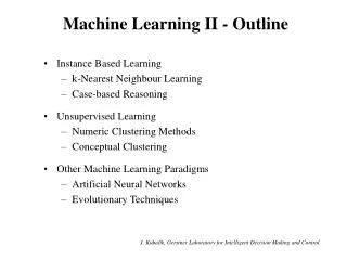
Machine LearningLecture outline 1 Learning in AI (machine learning) 2 Reinforcement learning 3 Learning in multi-agent systems 3.1 Learning action coordination 3.2 Learning individual performance 3.3 Learning to communicate 3.4 Layered learning 5 Conclusions
1 Learning in AI • What is machine learning? Herbet Simon defines learning as: “any change in a system that allows it to perform better the second time on repetition of the same task or another task drawn from the same population (Simon, 1983).” In ML the agent learns: • knowledge representation of the problem domain • problem solving rules, inferences • problem solving strategies 3
Classifying learning In MAS learning the agents should learn: • what an agent learns in ML but in the context of MAS - both cooperative and self-interested agents • how to cooperate for problem solving - cooperative agents • how to communicate - both cooperative and self-interested agents • how to negotiate - self interested agents Different dimensions • explicitly represented domain knowledge • how the critic component (performance evaluation) of a learning agent works • the use of knowledge of the domain/environment 4
Agents State and goals goal : E {0, 1} Utilities utility : E R env : E x A P(E) Expected utility of an action a in a state e Maximum Expected Utility (MEU) 5
Teacher Single agent learning Learning Process Feed-back Data Environment Learning results Problem Solving K & B Inferences Strategy Feed-back Results Performance Evaluation 6
Learning Process Learning results Problem Solving K & B Self Inferences Other Strategy agents Results Agent Agent Agent Performance Evaluation Self-interested learning agent Feed-back Communication Data NB: Both in this diagram and the next, not all components or flow arrows are always present - it depends on the type of agent (cognitive, reactive), type of learning, etc. Environment Actions Feed-back 7
Problem Solving K & B Self Inferences Other Strategy agents Problem Solving K & B Self Inferences Other Strategy agents Agent Agent Cooperative learning agents Feed-back Learning Process Feed-back Learning Process Communication Learning results Learning results Data Results Results Performance Evaluation Feed-back Actions Actions Communication Communication Environment 8
2 Reinforcement learning • Trial-and-error interactions with a dynamic environment • The feedback of the environment – reward or reinforcement • Learnutilitybased on statistical techniques and dynamic programming methods 9
E T s a I i R B r 2.1 A reinforcement-learning model B – agent's behavior i – input = current state of the env r – value of reinforcement (reinforcement signal) T – model of the world The model consists of: - a discrete set of environment states S (sS) - a discrete set of agent actions A (a A) - a set of scalar reinforcement signals, typically {0, 1} or real numbers - the transition model of the world, T • environment is nondeterministic T : S x A P(S) – T = transition model T(s, a, s’) 10
2.2 Features varying RL • accessible / inaccessible environment • has (T known) / has not a model of the environment • learn behavior / learn behavior + model • reward received only in terminal states or in any state • passive/active learner: • learn utilities of states • active learner – learn also what to do • how does the agent represent B, namely its behavior: • utility functions on states or state histories (T is known) • active-value functions (T is not necessarily known) - assigns an expected utility to taking a given action in a given state 11
2.3 The RL problem • the agent has to find a policy = a function which maps states to actions and which maximizes some long-time measure of reinforcement. • The agent has to learn an optimal behavior = optimal policy = a policy which yields the highest expected utility - * The utility function depends on the environment history (a sequence of states) In each state s the agents receives a reward - R(s) 12
Models of behavior • Finite-horizon model: at a given moment of time the agent should optimize its expected reward for the next h steps E(t=0, h R(st)) R(st) represents the reward received t steps into the future. • Infinite-horizon model: optimize the long-run reward E(t=0, R(st)) • Infinite-horizon discounted model: optimize the long-run reward but rewards received in the future are geometrically discounted according to a discount factor. E(t=0,t R(st)) 0 < 1. can be interpreted in several ways: an interest rate, a probability of living another step, or a mathematical trick to bound an infinite sum. 13
Markov Decision Problem (MDP) • The model is Markov if the state transitions are independent of any previous environment states or agent actions. • MDP: finite-state and finite-action – focus on that / infinite state and action space • Choose a policy ; choose the optimal policy * • For every MDP there exists an optimal policy • It’s a policy such that for every possible start state there is no better option than to follow the policy • Finding the optimal policy given a model T = calculate the utility of each state U(state) and use state utilities to select an optimal action in each state. 14
Bellman equation - U(s) • The utility of a state is the immediate reward for that state plus the expected discounted utility of the next state, assuming that the agent chooses the optimal action • U(s) = R(s) + max a [s’T(s,a,s’)*U(s’)] • The utility function U(s) allows the agent to select actions by using the Maximum Expected Utility principle *(s) = arg maxa (R(s) + s’T(s,a,s’)*U(s’)) optimal policy 15
+1 +1 -1 -1 A 4 x 3 environment • The intended outcome occurs with probability 0.8, and with probability 0.2 (0.1, 0.1) the agent moves at right angles to the intended direction. • The two terminal states have reward +1 and –1, all other states have a reward of –0.04, =1 0.8 0.1 0.1 3 2 1 3 2 1 0.812 0.868 0.918 0.762 0.660 0.705 0.655 0.611 0.388 1 2 3 4 1 2 3 4 16
+1 -1 Bellman equation for the 4x3 world Equation for the state (1,1) U(1,1) = -0.04 + max{ 0.8 U(1,2) + 0.1 U(2,1) + 0.1 U(1,1), Up 0.9U(1,1) + 0.1U(1,2), Left 0.9U(1,1) + 0.1U(2,1), Down 0.8U(2,1) +0.1U(1,2) + 0.1U(1,1)} Right Up is the best action 3 2 1 0.812 0.868 0.918 0.762 0.660 0.705 0.655 0.611 0.388 1 2 3 4
defines the best action in state s Value Iteration • Given the maximal expected utility, the optimal policy is: *(s) = arg maxa(R(s) + s’ T(s,a,s’) * U(s’)) • Compute U*(s) using an iterative approach Value Iteration U0(s) = R(s) Ut+1(s) = R(s) + maxa(s’ T(s,a,s’) * Ut(s’)) t inf ….utility values converge to the optimal values compute for all s 18
Policy iteration Manipulate the policy directly, rather than finding it indirectly via the optimal value function • choose an arbitrary policy (randomly) • at each time t, compute the long time reward starting in s, using t, i.e. solve the equations Ut(s) = R(s) + s’ (T(s, t(s),s’) * Ut(s’)) • improve the policy at each state t+1(s) arg maxa (R(s) + s’ T(s,a,s’) * Ut(s’)) 19
2.6 RL learning • Use observed rewards to learn an optimal (or near optimal) policy for the environment Ex: play 100 moves, you loose • In an MDP the agent has a complete model of the environment • Now the agent has not such a model • (a) Passive learning – the agent policy is fixed • The task is to learn the utilities of states (or state-action pairs) • (b) Active learning – the agent must also learn what to do: exploitation/exploration 20
(a) Passive reinforcement learning • Policy is fixed = in state s always execute (s) • Goal – learn how good the policy is = learn U(s) • Does not know T(s,a,s’), does not know before R(s) ADP (Adaptive Dynamic Programming) learning The problem of calculating an optimal policy in an accessible, stochastic environment. ADP = plug the learned T(s, (s),s’) and the observed rewards R(s) into the Bellman equations to calculate the utility of states Supervised learning – input: state-action pairs output: resulting state Estimate transition probabilities T(s,a,s’) from frequencies with which s’ is reached after executing a in s’ (1,3) – Right – 2 times (2,3), 1 time in (1,3) => T((1,3), Right, (2,3)) = 2/3 21
Temporal difference learning (TD learning) The value function is no longer implemented by solving a set of linear equations, but it is computed iteratively. • Used observed transitions to adjust the values of the observed states so that they agree with the constraint equations. U(s) U (s) + (R(s) + U (s’) – U (s)) is the learning rate. • Whatever state is visited, its estimated value is updated to be closer to R(s) + U (s’) since R(s) is the instantaneous reward received and U (s') is the estimated value of the actually occurring next state. • simpler, involves only next states • decreases as the number of times the state is visited increases 22
Temporal difference learning • Does not need a model to perform its updates • The environment supplies the connections between neighboring states in the form of observed transitions. ADP and TD comparison • ADP and TD try both to make local adjustments to the utility estimates in order to make each state « agree » with its successors • TD adjusts a state to agree with the observed successor • ADP adjusts a state to agree with all of the successors that might occur, weighted by their probabilities 23
(b) Active reinforcement learning • Passive learning agent – has a fixed policy that determines its behavior • An active learning agent must decide what action to take • The agent must learn a complete model with outcome probabilities for all actions (instead of a model for the fixed policy) • Compute/learn the utilities that obey the Bellman equation U (s) = R(s) + maxas’ (T(s, t(s),s’) * U(s’)) using value iteration or policy iteration 24
Active reinforcement learning • If value iteration then look for the action that maximzes utility • If policy iteration you already have the action • Exploration/exploitation • The representative problem is the n-armed bandit problem Solutions • 1/n time choose random actions, rest follow • give weights to actions that have not been explored, avoid actions with low utilities • Exploratory function –– how greedy : prefer high utility values (exploitation) or not (exploration) 25
Q-learning Active learning of action-value functions action-value function = assigns an expected utility to taking a given action in a given state, Q-values Q(a, s)– the value of doing action a in state s (expected utility) Q-values are related to utility values by the equation: U(s) = maxaQ(a, s) • Approach 1 Q(a,s) = R(s) + s’(T(s,a,s’) *maxa’ Q(a’,s’)) This requires a model • Approach 2 Use TD The agent does not need to learn a model – model free 26
Q-learning TD learning, unknown environment Q(a,s) Q(a,s) + (R(s) + maxa’Q(a’, s’) – Q(a,s)) calculated after each transition from state s to s’. • Is it better to learn a model and a utility function or to learn an action-value function with no model? 27
Q-learning function Q-Learning-Agent(percept) returns an action inputs: percept, a percept indicating the current state s’ and reward signal r’ variable: Q, a table of action values index by state and action Nsa, a table of frequencies for state-action pairs s, a, r the previous state, action, and reward, initially null if s is not null then increment Nsa[s,a] Q[a,s] Q[a,s] + (Nsa[s,a])(r + maxa’Q [a’,s’] – Q [a,s]) if Terminal[s’] then s, a, r null else s, a, r` s’, argmaxa’ f(Q[a’, s’], Nsa[a’,s’]), r’ return a end s, a, r` s’, argmaxa’ (Q[a’, s’]), r’ 28
Generalization of RL • The problem of learning in large spaces – large no. of states • Generalization techniques - allow compact storage of learned information and transfer of knowledge between "similar" states and actions. • Neural nets • Decision trees • U(state)=U(most similar sate in memory) • U(state) =average U(most similar sates in memory) 29
3 Learning in MAS • The credit-assignment problem (CAP) = the problem of assigning feed-back (credit or blame) for an overall performance of the MAS (increase, decrease) to each agent that contributed to that change • inter-agent CAP = assigns credit or blame to the external actions of agents • intra-agent CAP = assigns credit or blame for a particular external action of an agent to its internal inferences and decisions • distinction not always obvious 30
3.1 Learning action coordination • s – current environment state • Agent i – determines the set of actions (j) it can do in s: Ai(s) = {Aij(s)} • Computes the goal relevance of each action: Eij(s) • Agent i announces a bid for each action with Eij(s) > threshold • Bij(s) = ( + ) Eij(s) • - risk factor (small) - noise term (to prevent convergence to local minima) 31
The action with the highest bid is selected • Incompatible actions are eliminated • Repeat process until all actions in bids are either selected or eliminated • A – selected actions = activity context • Execute selected actions • Update goal relevance for actions in A Eij(s) Eij(s) – Bij(s) + (R / |A|) R –external reward received • Update goal relevance for actions in the previous activity context Ap (actions Akl) Ekl(sp) Ekl(sp) + (AijA Bij(s)/ |Ap|) 32
3.2 Learning individual performance The agent learns how to improve its individual performance in a multi-agent settings Examples • Cooperative agents - learning organizational roles • Competitive agents - learning from market conditions 33
3.2.1 Learning organizational roles(Nagendra, e.a.) • Agents learn to adopt a specific role in a particular situation (state) in a cooperative MAS. • Aim = to increase utility of final states • Each agent may play several roles in a situation • The agents learn to select the most appropriate role • Use reinforcement learning • Utility, Probability, and Cost (UPC) estimates of a role in a situation • Utility - the agent's estimate of a final state worth for a specific role in a situation – world states mapped to smaller set of situations S = {s0,…,sf} Urs = U(sf), s0 … sf 34
Probability - the likelihood of reaching a final state for a specific role in a situation Prs = p(sf), s0 … sf • Cost - the computational cost of reaching a final state for a specific role in a situation • Potential of a role - estimates the usefulness of a role, depending on global information and constraints • Representation: • Sk - vector of situations for agent k, SK1,…,SKn • Rk - vector of roles for agent k, Rk1,…,Rkm • |Sk| x |Rk| x 4 values to describe UPC and Potential 35
Functioning Phase I: Learning Several learning cycles; in each cycle: • each agent goes from s0 to sf and selects its role as the one with the highest probability Probability of selecting a role r in a situation s f - objective function used to rate the roles (e.g., f(U,P,C,Pot) = U*P*C + Pot) - depends on the domain 36
Use reinforcement learning to update UPC and the potential of a role • For every s [s0,…,sf] and chosen role r in s Ursi+1 = (1-)Ursi + Usf i - the learning cycle Usf - the utility of a final state 01 - the learning rate Prsi+1 = (1-)Prsi + O(sf) O(sf) = 1 if sf is successful, 0 otherwise 37
Potrsi+1 = (1-)Potrsi + Conf(Path) Path = [s0,…,sf] Conf(Path) = 0 if there are conflicts on the Path, 1 otherwise • The update rules for cost are domain dependent Phase II: Performing In a situation s the role r is chosen such that: 38
3.2.2 Learning in market environments(Vidal & Durfee) Agents use past experience and evolved models of other agents to better sell and buy goods • Environment = a market in which agents buy and sell information (electronic marketplace) • Open environment • The agents are self-interested (max local utility) {g} - a set of goods P - set of possible prices for goods Qg - set of possible qualities for a good g 39
information has a cost for the seller and a value for the buyer • information is sold at a certain price • a buyer announces a good it needs • sellers bid their prices for delivering the good • the buyer selects from these bids and pays the corresponding price • the buyer assesses the quality of information after it receives it from the seller • Profit of a seller s for selling the good gat price p Profitsg(p) = p - csg csg - the cost of producing the good g by s; p - the price • Value of a good g for a buyer b Vbg(p,q) p - price b paid for g q - quality of good g Goal seller - maximize profit in a transaction buyer - maximize value in a transaction 40
3 types of agents 0-level agents • they set their buying and selling prices based on their own past experience • they do not model the behavior of other agents 1-level agents • model other agents based on previous interactions • they set their buying and selling prices based on these models and on past experience • they model the other agents as 0-level agents 2-level agents • same as 1-level agents but they model the other agents as 1-level agents 41
Strategy of 0-level agents 0-level buyer - learns the expected value function, fg(p), of buying g at price p - uses reinforcement learning fgi+1(p) = (1-)fgi(p) + Vbg(p,q),min 1, for i=0, = 1 - chooses the seller s* for supplying a good g 0-level seller - learns the expected profit function, hg(p), if it offers good g at price p - uses reinforcement learning hgi+1(p) = (1-)hgi(p) + Profitbg(p) where Profitbg(p) = p - csg if it wins the auction, 0 otherwise - chooses the price ps* to sell the good g so as to maximize profit 42
Strategy of 1-level agents 1-level buyer - models sellers for good g - does not model other buyers - uses a probability distribution functionqsg(x) over the qualities x of a good g - computes expected utility, Esg, of buying good g from seller s - chooses the seller s* for supplying a good g that maximizes this expected utility 43
1-level seller - models buyers for good g - models the other sellers s for good g • Buyer's modeling - uses a probability distribution function mbg(p) - the probability that b will choose price p for good g • Seller's modeling - uses a probability distribution function ns'g(y) - the probability that s' will bid price y for good g - computes the probability of bidding lower than a given seller s' with the price p Prob_of_bidding_lower_than_s' = p'(Prob of bid of s' with p' for which s wins) = p' N(g,b,s;s',p,p') N(g,b,s;s',p,p') = ns'g(p') if mbg(p') mbg(p) 0 otherwise 44
- computes the probability of bidding lower than all other sellers with the price p Prob_of_bidding_lower_with_p = (Prob_of_bidding_lower_than_s') s'S - {s} - chooses the best price p* to bid so as to maximize profit 45
3.3 Learning to communicate • What to communicate (e.g., what information is of interest to the others) • When to communicate (e.g., when try doing something by itself or when look for help) • With which agents to communicate • How to communicate (e.g., language, protocol, ontology) 46
Learning with which agents to communicate(Ohko, e.a. ) • Learning to which agents to ask for performing a task • Used in a contract net protocol for task allocation to reduce communication for task announcement • Goal = acquire and refine knowledge about other agents' task solving abilities • Case-based reasoning used for knowledge acquisition and refinement A case consists of: (1) A task specification (2) Information about which agents solved a task or similar tasks in the past and the quality of the provided solution 47
(1)Task specification Ti = {Ai1 Vi1, …, Aimi Vimi} Aij - task attribute, Vij - value of attribute • Similar tasks Sim(Ti, Tj) = r s Dist(Air, Ajs) AirTi, AjsTj Dist(Air, Ajs) = Sim_Attr(Air, Ajs) * Sim_Vals(Vir, Vjs) • Set of similar tasks S(T) = {Tj : Sim(T, Tj) 0.85} 48
(2)Which agents performed T or similar tasks in the past Suitability of Agent k Perform(Ak, Tj) - quality of solution for Tj assured by agent Ak performing Tj in the past • The agent computes { Suit(Ak, T), Suit(Ak, T)>0 } and selects the agent k* such that or the first m agents with best suitability • After each encounter, the agent stores the tasks performed by other agents and the solution quality • Tradeoff between exploitation and exploration 49
3.4 Layered learning (Stone & Veloso) • A hierarchical machine learning paradigm in MAS • Used simulated robotic soccer – RoboCup Learning Input Output – Intractable • Decompose the learning task L into subtasks: L1, …, Ln • Characteristics of the environment: • Cooperative MAS • Teammates and adversaries • Hidden states – agents have a partial world view at any given moment • Agents have noisy sensory data and actuators • Perception and action cycles are asynchronous • Agents must make their decisions in real-time 50