From Linear
IAPT Workshop. 2 nd August ISP, CUSAT. From Linear. Nonlinear Physics. To. V P N Nampoori nampoori@gmail.com. Simple pendulum. Oscillate. Rotate. Simple pendulum. Oscillate. Rotate. Double pendulum. Taking the amplitude small. θ. The hallmark of linear equations.
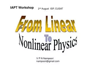

From Linear
E N D
Presentation Transcript
IAPT Workshop 2nd August ISP, CUSAT From Linear Nonlinear Physics To V P N Nampoori nampoori@gmail.com
Simple pendulum Oscillate Rotate
Simple pendulum Oscillate Rotate Double pendulum
Taking the amplitude small θ
The hallmark of linear equations. We can predict state of the simple pendulum at any future time Linearlty helps us to predict future.
Alternate representation of damped motion of simple pendulum Phase space plot
Second order nonlinear differential equation Superposition principle is not valid Prediction is not possible
One-dimensional maps One-dimensional maps, definition: - a set V (e.g. real numbers between 0 and 1) - a map of the kind f:VV Linear maps: - a and b are constants - linear maps are invertible with no ambiguity Non-linear maps: The logistic map
Motivation: Discretization of the logistic equation for the dynamics of a biological population x b: birth rate (assumed constant) cx: death rate depends on population (competition for food, …) How do we explore the logistic map? One-dimensional maps Non-linear maps: The logistic map with
Evolution of the logistic map fixed point ? Geometric representation 1 Evolution of a map: 1) Choose initial conditions 2) Proceed vertically until you hit f(x) 3) Proceed horizontally until you hit y=x 4) Repeat 2) 5) Repeat 3) . : x f(x) 0 0.5 1
1 1 y=x y=x f(x) f(x) 0 0.5 1 0 0.5 1 1 1 0 0.5 1 0 0.5 1 b) a) Phenomenology of the logistic map fixed point fixed point c) d) chaos? 2-cycle? What’s going on? Analyze first a) b) b) c) , …
1 1 x x f(x) f(x) 0 0.5 1 0 0.5 1 Geometrical representation Evolution of the logistic map fixed point How do we analyze the existence/stability of a fixed point?
Stability - Define the distance of from the fixed point Taylor expansion - Consider a neighborhood of - The requirement implies Logistic map? - Condition for existence: Fixed points - Logistic map: - Notice: since the second fixed point exists only for
1 1 x x f(x) f(x) 0 1 0.5 0 0.5 1 - Stability condition: Stability and the Logistic Map - First fixed point: stable (attractor) for - Second fixed point: stable (attractor) for • No coexistence of 2 stable fixed points for these parameters • (transcritical biforcation) What about ?
1 Observations: Period doubling x 1) The map oscillates between two values of x f(x) 0 0.5 1 0 0.5 1 Evolution of the logistic map 2) Period doubling: What is it happening?
0 0.5 1 These points form a 2-cycle for However, the relation suggests they are fixed points for the iterated map Stability analysis for : and thus: For , loss of stability and bifurcation to a 4-cycle Now, graphically.. • - At the fixed point becomes unstable, • since • Observation: an attracting 2-cycle starts • (flip)-bifurcation • The points are found solving the equations > Period doubling and thus: Why do these points appear?
Plot of fixed points vs Bifurcation diagram
International Relations and Logistic Map Let A and B are two neighbouring countries Both countries look each other with enmity. Country A has x1 fraction of the budget for the Defence for year 1 Country B has same fraction in its budget as soon as A’s budget session Is over Next year A has increased budget allocation x2 Budget allocation goes on increasing. If complete budget is for Defence , it is not possible since no funds for Other areas
1 x f(x) 0 0.5 1 Fund allocation for subsequent years for the country A As time progresses, budget allocation for defense decreases. Peace time . A and B are friends.
Parameter μ is called enmity parameter. Now let a third country C intervenes In the region to modulate the enmity parameter and μ = μ(t)
1 1 y=x y=x f(x) f(x) 0 0.5 1 0 0.5 1 1 1 0 0.5 1 0 0.5 1 b) a) Phenomenology of the logistic map fixed point fixed point c) d) chaos? 2-cycle? What’s going on? Analyze first a) b) b) c) , …
1 1 x x f(x) f(x) 0 1 0.5 0 0.5 1 Budget allocation stabilises To a fixed value. Caution time. Yellow Budget allocation decreases and goes to zero Full peace time Green
1 Observations: Period doubling x 1) The map oscillates between two values of x f(x) 0 0.5 1 0 0.5 1 Evolution of the logistic map 2) Period doubling: What is it happening?
Plot of fixed points vs Tension builds up Bifurcation diagram Peace time WAR!!!
Evolution of International Relationships between three countries Two countries are at enmity and the third is the controlling country From Peace time to War time
Interaction leads to modification of dynamics. A, B and C are three components of a system with two states YES (1) or NO ( 0) Case 1 A, B and C are non interacting Following are the 8 equal probable states of the system 1=( 000), 2=( 001), 3=(010), 4=( 100),5=(110),6=(101),7=(011), 8=(111) Probability of occurrence is 1/8 for all the states. States evolve randomly. Case II Let A obeys AND logic gate while B and C obey OR logic gate
T2 T3 T1 1/8 I (000) (000) (000) (000) (001) (010) (001) (010) II bistable (010) 2/8 (001) (001) (010) (111) (111) (100) (011) (111) (111) (011) III 5/8 (110) (111) (111) Evolution to Fixed state Blissful state!!! (101) (011) (111) (111) (111) (011) (111) (111) (111) (111)
Photograph of melting ice landscape – Face of Jesus Christ - evolution leading to fixed state
Linear Optics Maxwell’s Equations : Light -- Matter Interaction Maxwell’s equations for charge free, nonmagnetic medium .D = 0 .B = 0 XE = -B/t XH = D/t D = 0E + P and B = 0H In vacuum, P = 0 and on combining above eqns 2E - 00 2 E/t2 = 0 or 2E - 1/c22 E/t2 = 0 In a medium, 2E - 00 2 E/t2 - 02P/t2 = 0 writing P = 0 E, 2E - 1/v22 E/t2 = 0 where, v = (0 )-1/2 Defining c/v = n, 2E - n2/c22 E/t2 = 0 we get a second order linear diffl eqn describing what is called, Linear Optics
P=(1) E + (2) E2 + (3)E3 +….. (n)/ (n+1) << 1 For isotropic medium, (n) will be scalar. (n) represents nth order non linear optical coefficient
Polarisation of a medium P = PL +PNL where,PL = (1) E andPNL = (2)E2 + (3)E3+….. On substituting P in the Maxwell’s eqns, we get 2E - n2/c22 E/t2 = 02PNL/t2 This is nonlinear differential equation and describes various types of Nonlinear optical phenomena. Type of NL effects exhibited by the medium depend the order of nonlinear optical coefficient. E Polarisation Maxwell’s eqns feedback
2 Optical second harmonic generation 1 3 2 Sum (difference) frequency generation OPC by DFWM
Consequence of 3rd order optical nonlinearity intensity dependent complex refractive index
One of the consequences of 3rd order NL PNL = (1)E + (3)E3 =( (1) + (3)E2)E = (n1 + n2 I)E We have n(I) = (n1 + n2 I) n2< 0 n n1 n2> 0 I Intensity dependent ref.index has applications in self induced transparency, self focussing, optical limiting and in optical computing.
α T I Saturable absorbers– Materials which become transparent above threshold intense light pulses Materials become transparent at high intensity Absorption decreases with intensity Is
It I Optical Limiters : Materials which are opaque above a threshold laser intensity Materials become opaque at higher intensity Is
Materials become opaque at higher pump intensity – optical limiter Materials become transparent at higher pump intensity- saturable absorber
Optical limiters are used in…… • Protection of eyes and sensitive devices from intense light pulses • Laser mode locking • Optical pulse shaping • Optical signal processing and computing .
Intensity dependent refractive index Laser beam :Gaussian beam I(r ) = I0exp(-2r2/w2) I(r ) Beam cross section r