Download
1 / 25
260 likes | 467 Vues
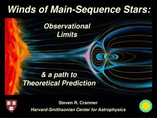
Winds of Main-Sequence Stars:. Observational Limits. & a path to Theoretical Prediction. Steven R. Cranmer Harvard-Smithsonian Center for Astrophysics. Winds of Main-Sequence Stars:. Outline: Background: the solar wind ( M ~ 10 –14 M /yr)

E N D
Winds of Main-Sequence Stars: Observational Limits & a path toTheoretical Prediction Steven R. CranmerHarvard-Smithsonian Center for Astrophysics
Winds of Main-Sequence Stars: • Outline: • Background: the solar wind (M ~ 10–14M /yr) • Cool-star winds: observational M methods & results • How can theory be folded in? Should it be? Steven R. CranmerHarvard-Smithsonian Center for Astrophysics
Brief history: solar wind • Mariner 2 (1962): first direct confirmation of continuous supersonic solar wind. • Helios probed in to 0.3 AU, Voyager continues past 100+ AU. • Ulysses (1990s) left the ecliptic; provided 3D view of the wind’s magnetic geometry.
Brief history: solar wind • Mariner 2 (1962): first direct confirmation of continuous supersonic solar wind. • Helios probed in to 0.3 AU, Voyager continues past 100+ AU. • Ulysses (1990s) left the ecliptic; provided 3D view of the wind’s magnetic geometry. • SOHO gave us new views of “source regions” of solar wind.
The solar wind mass los rate • The sphere-averaged “M” isn’t usually considered by solar physicists! • Wang (1998, CS10) used empirical relationships between B-field, wind speed, and density to reconstruct M over two solar cycles. ACE (in ecliptic)
AGB Pre-MS HB ZAMS Mass loss over the Sun’s lifetime • T Tauri phase: Does accretion drive wind? (Matt & Pudritz 2005) • ZAMS: Was there a “bright young Sun?” • HB/AGB: Is mass loss the “2nd parameter?” Do winds clear out “missing ISM” in clusters? • Close binaries: SN Ia properties!
Cool-star winds: “traditional” diagnostics • Optical/UV spectroscopy: simple blueshifts or full “P Cygni” profiles • IR continuum: circumstellar dust causes SED excess • Molecular lines (mm, sub-mm): CO, OH maser • Radio: free-free emission from (partially ionized?) components of the wind • Continuum methods need V from another diagnostic to get mass loss rate. • Clumping? (Bernat 1976) wind star (van den Oord & Doyle 1997)
Cool-star mass loss rates de Jager et al. (1988)
Multi-line spectroscopy • 1990s: more self-consistent treatments of radiative transfer AND better data (GHRS, FUSE, high-spectral-res ground-based) led to better stellar wind diagnostic techniques! • A nice example: He I 10830 Å for TW Hya (pole-on T Tauri star) . . . Dupree et al. (2006)
Hartigan et al. (1995) Carpenter, Harper, Dupree, etc. Cool-star mass loss rates de Jager et al. (1988)
New ideas (1): astrosphere absorption • Wood et al. (2001, 2002, 2005) distinguished cool ISM H I Lyα absorption from hotter “piled up” H0 in stellar astrospheres. Derived M depends on models . . .
New ideas (2): accretion in pre-CVs • Some H-rich & He-rich white dwarfs show metal lines in their atmospheres (classes DAZ, DZ). Accretion from ISM and/or “comets” is problematic. • Debes (2006) suggested that M-dwarf companions deposit metal-rich gas via stellar winds onto the WD surfaces. • Observed abundances (usually from Ca H, K lines) modeled as steady-state balance between accretion & downward diffusion; this provides Macc ; • Bondi-Hoyle accretion rate provides the density; • Mass conservation (spherical geometry) provides Mwind . • Largest uncertainty: wind velocity (v4).
Wood et al. (2005) Debes (2006) Cool-star mass loss rates
100x M New ideas (3): charge exchange X-rays • ISM neutrals flow into an “astrosphere” and CX with wind ions. • Ions left in excited state emit X-rays. • Wargelin & Drake (2001, 2002) suggest using this to probe stellar wind properties. • So far, upper limits only (M dwarfs). • Better spatial & spectral res. needed. • With good enough spectra, one can also obtain wind speed, composition, and ionization state.
Theory: dimensional analysis . . . • Stellar wind power: • Reimers (1975, 1977) proposed a semi-empirical scaling:
Theory: dimensional analysis . . . • Stellar wind power: • Reimers (1975, 1977) proposed a semi-empirical scaling: • Schröder & Cuntz (2005) investigated an explanation via convective turbulence generating atmospheric waves . . . • Funny things happen during rapid evolutionary stages! (e.g., Willson 2000, Ann. Rev.)
Schröder & Cuntz (2005) scaling for I, III, V Cool-star mass loss rates
heat conduction radiation losses 5 2 — ρvkT What sets solar mass loss? • Coronal heating must be ultimately responsible! • Hammer (1982) & Withbroe (1988) suggested a steady-state energy balance: • Only a fraction of total coronal heat flux conducts down, but in general, we expect something close to . . . along open flux tubes!
open or closed fields? K, M stars Sun Stellar coronal heating • The well-known “rotation-age-activity” relationship shows how coronal heating weakens as young (solar-type) stars spin down. • Heating rates also scale with mean magnetic field. Judge, Güdel, Kürster, Garcia-Alvarez, Preibisch, Feigelson, Jeffries Saar (2001, CS11)
Solar X-rays & magnetic flux • Empirically, does solar mass loss really scale with FX ~ Φ ? It depends on which field lines are considered! Coronal hole (open) Quiet regions Schwadron et al. (2006) Active regions
Solar X-rays & magnetic flux • Empirically, does solar mass loss really scale with FX ~ Φ ? It depends on which field lines are considered! M ~ ΦAR0.06 M ~ ΦQR0.41 Active regions Quiet regions Schwadron et al. (2006)
Sun’s mass loss history • Did liquid water exist on Earth 4 Gyr ago? If “standard” solar models are correct, a strong greenhouse effect was needed. • Sackmann & Boothroyd (2003) argued that a more massive (~1.07 M) young Sun could have been luminous enough to solve this problem, but it would have needed strong early mass loss . . . Sackmann & Boothroyd (2003) M ~ LX1.3 M ~ LX1.0 M ~ LX0.4 M ~ LX0.1
Z– Z+ Z– Heating & wind acceleration • Models of how coronal heating (FX) scales with magnetic flux (Φ) are growing more sophisticated . . . • Closed loops: Magnetic reconnection e.g., Longcope & Kankelborg 1999 • Open field lines: MHD turbulence! T (K) reflection coefficient Cranmer & van Ballegooijen (2005, 2007) T. Suzuki (CS14, Poster II)
Conclusions Observations: • Combined multi-ion spectroscopy & atmosphere modeling still has unexplored potential. • Magnetic field measurements are also key to constraining stellar wind properties. ZDI! • Coming soon: X-ray charge exchange M’s ? Theory: • Understanding mass loss depends on modeling coronal heating on open & closed field lines. • Coming soon: 3D convection simulations for rapid rotators, with implications for how the photospheric waves affect coronal heating . . . • Here now: turbulence-driven wind models with “real” coronal heating! B. Brown et al. (2004)