Automated Black-Box Optimization for Real-World Problem Solving
710 likes | 806 Vues
This article explores employing meta-heuristic black-box optimization algorithms, such as BBSAs, to solve complex real-world problems. It addresses the practitioner's dilemma, theory-practice gap, and the need for a scalable solution enabling routine problem-solving. The paper presents methods for solving single-instance and multiple-instance problems, automated BBSA selection, configuration, and result interpretation. Additionally, it discusses coevolution, self-adaptation, and self-configuring crossover techniques. Experimental results demonstrate successful application in various scenarios.

Automated Black-Box Optimization for Real-World Problem Solving
E N D
Presentation Transcript
Automated real-world problem solving EMPLOYING meta-heuristicalblack-box optimization Daniel R. Tauritz, Ph.D. Guest Scientist, Los Alamos National Laboratory Director, Natural Computation Laboratory Department of Computer Science Missouri University of Science and Technology
Black-Box Search Algorithms • Many complex real-world problems can be formulated as generate-and-test problems • Black-Box Search Algorithms (BBSAs) iteratively generate trial solutions employing solely the information gained from previous trial solutions, but no explicit problem knowledge
Practitioner’s Dilemma • How to decide for given real-world problem whether beneficial to formulate as black-box search problem? • How to formulate real-world problem as black-box search problem? • How to select/create BBSA? • How to configure BBSA? • How to interpret result? • All of the above are interdependent!
Theory-Practice Gap • While BBSAs, including EAs, steadily are improving in scope and performance, their impact on routine real-world problem solving remains underwhelming • A scalable solution enabling domain-expert practitioners to routinely solve real-world problems with BBSAs is needed
Two typical real-world problem categories • Solving a single-instance problem: automated BBSA selection • Repeatedly solving instances of a problem class: evolve custom BBSA
Part I: Solving Single-Instance Problems Employing Automated BBSA Selection
Requirements • Need diverse set of high-performance BBSAs • Need automated approach to select most appropriate BBSA from set for a given problem • Need automated approach to configure selected BBSA
Automated BBSA Selection • Given a set of BBSAs, a priori evolve a set of benchmark functions which cluster the BBSAs by performance • Given a real-world problem, create a surrogate fitness function • Find the benchmark function most similar to the surrogate • Execute the corresponding BBSA on the real-world problem
A Priori, Once Per BBSA Set Benchmark Generator BBSA1 BBSA2 … BBSAn BBSAn BBSA1 BBSA2 BPn BP1 BP2 …
A Priori, Once Per Problem Class Real-World Problem Sampling Mechanism Surrogate Objective Function Match with most “similar” BPk Identified most appropriate BBSAk
Per Problem Instance Real-World Problem Sampling Mechanism Surrogate Objective Function Apply a priori established most appropriate BBSAk
Requirements • Need diverse set of high-performance BBSAs • Need automated approach to select most appropriate BBSA from set for a given problem • Need automated approach to configure selected BBSA
Static vs. dynamic parameters • Static parameters remain constant during evolution, dynamic parameters can change • Dynamic parameters require parameter control • The optimal values of the strategy parameters can change during evolution [1]
Solution Create self-configuring BBSAs employing dynamic strategy parameters
Self Adaptation • Dynamical Evolution of Parameters • Individuals Encode Parameter Values • Indirect Fitness • Poor Scaling
Coevolution Basics Def.: In Coevolution, the fitness of an individual is dependent on other individuals (i.e., individuals are part of the environment) Def.: In Competitive Coevolution, the fitness of an individual is inversely proportional to the fitness of some or all other individuals
Supportive Coevolution • Primary Population • Encodes problem solution • Support Population • Encodes configuration information Support Individual Primary Individual
Multiple Support Populations • Each Parameter Evolved Separately • Propagation Rate Separated
Benchmark Functions • Rastrigin • Shifted Rastrigin • Randomly generated offset vector • Individuals offset before evaluation
Fitness Results • All Results Statistically Significantaccording to T-test with α = 0.001
Conclusions • Proof of Concept Successful • SuCo outperformed SA on all but on test problem • SuCo Mutation more successful • Adapts better to change in population fitness
Motivation • Performance Sensitive to Crossover Selection • Identifying & Configuring Best Traditional Crossover is Time Consuming • Existing Operators May Be Suboptimal • Optimal Operator May Change During Evolution
Some Possible Solutions • Meta-EA • Exceptionally time consuming • Self-Adaptive Algorithm Selection • Limited by algorithms it can choose from
Self-Configuring Crossover (SCX) Offspring Crossover • Each Individual Encodes a Crossover Operator • Crossovers Encoded as a List of Primitives • Swap • Merge • Each Primitive has three parameters • Number, Random, or Inline Swap(3, 5, 2) Merge(1, r, 0.7) Swap(r, i, r)
Applying an SCX Concatenate Genes 1.0 5.0 2.0 6.0 3.0 7.0 4.0 8.0 Parent 1 Genes Parent 2 Genes
The Swap Primitive • Each Primitive has a type • Swap represents crossovers that move genetic material • First Two Parameters • Start Position • End Position • Third Parameter Primitive Dependent • Swaps use “Width” Swap(3, 5, 2)
Applying an SCX Concatenate Genes 1.0 5.0 2.0 6.0 3.0 7.0 4.0 8.0 Offspring Crossover Swap(3, 5, 2) 3.0 4.0 5.0 6.0 Merge(1, r, 0.7) Swap(r, i, r)
The Merge Primitive • Third Parameter Primitive Dependent • Merges use “Weight” • Random Construct • All past primitive parameters used the Number construct • “r” marks a primitive using the Random Construct • Allows primitives to act stochastically Merge(1, r, 0.7)
Applying an SCX Concatenate Genes 3.0 1.0 2.0 4.0 5.0 7.0 8.0 6.0 Offspring Crossover Swap(3, 5, 2) 0.7 g(i) = α*g(i) + (1-α)*g(j) Merge(1, r, 0.7) g(1) = 1.0*(0.7) + 6.0*(1-0.7) g(2) = 6.0*(0.7) + 1.0*(1-0.7) 2.5 4.5 Swap(r, i, r)
The Inline Construct • Only Usable by First Two Parameters • Denoted as “i” • Forces Primitive to Act on the Same Loci in Both Parents Swap(r, i, r)
Applying an SCX Concatenate Genes 2.5 3.0 2.0 4.0 5.0 7.0 4.5 8.0 Offspring Crossover 2.0 4.0 Swap(3, 5, 2) Merge(1, r, 0.7) Swap(r, i, r)
Applying an SCX Remove Exess Genes Concatenate Genes 2.5 3.0 4.0 2.0 5.0 7.0 4.5 8.0 Offspring Genes
Evolving Crossovers Parent 2 Crossover Parent 1 Crossover Offspring Crossover Swap(r, 7, 3) Swap(3, 5, 2) Merge(i, 8, r) Swap(4, 2, r) Merge(1, r, 0.7) Merge(r, r, r) Swap(r, i, r)
Empirical Quality Assessment • Compared Against • Arithmetic Crossover • N-Point Crossover • Uniform Crossover • On Problems • Rosenbrock • Rastrigin • Offset Rastrigin • NK-Landscapes • DTrap
SCX Overhead • Requires No Additional Evaluation • Adds No Significant Increase in Run Time • All linear operations • Adds Initial Crossover Length Parameter • Testing showed results fairly insensitive to this parameter • Even worst settings tested achieved better results than comparison operators
Conclusions • Remove Need to Select Crossover Algorithm • Better Fitness Without Significant Overhead • Benefits From Dynamically Changing Operator
Current Work • Combining Support Coevolution and Self-Configuring Crossover by employing the latter as a support population in the former [4]
Part II: Repeatedly Solving Problem Class Instances By Evolving Custom BBSAs Employing Meta-GP [5]
Problem • Difficult Repeated Problems • Cell Tower Placement • Flight Routing • Which BBSA, such as Evolutionary Algorithms, Particle Swarm Optimization, or Simulated Annealing, to use?
Possible Solutions • Automated Algorithm Selection • Self-Adaptive Algorithms • Meta-Algorithms • Evolving Parameters / Selecting Operators • Evolve the Algorithm
Our Solution • Evolving BBSAs employing meta-Genetic Programming (GP) • Post-ordered parse tree • Evolve a repeated iteration
Initialization Check for Termination Iteration Terminate
Our Solution • Genetic Programing • Post-ordered parse tree • Evolve a repeated iteration • High-level operations
Parse Tree • Iteration • Sets of Solutions • Root returns ‘Last’ set
Nodes: Variation Nodes • Mutate • Mutate w/o creating new solution (Tweak) • Uniform Recombination • Diagonal Recombination
Nodes: Selection Nodes • k-Tournament • Truncation
Nodes: Set Nodes • makeSet • Persistent Sets