Download
1 / 1
10 likes | 137 Vues
Iron perturbation 180m. Iron perturbation 270m. control. .03. .01. .07. 45 m. 154°-158 ° E, 0.5°S-0.5°N. .06. .03. .48. 95 m. .43. .08. .67. 142 m. .59. .44. 1.44. Mackey et al, 2002. 217 m. .20. 1.38. 6.24. 272 m. 160 E. 180W. 135W. 90W.

E N D
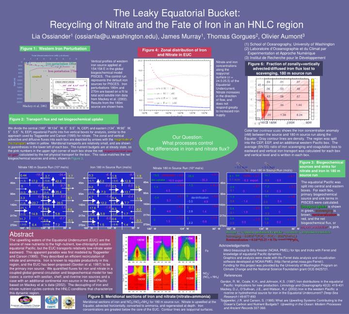
Iron perturbation 180m Iron perturbation 270m control .03 .01 .07 45 m 154°-158°E, 0.5°S-0.5°N .06 .03 .48 95 m .43 .08 .67 142 m .59 .44 1.44 Mackey et al, 2002 217 m .20 1.38 6.24 272 m 160E 180W 135W 90W Nitrate 180 m Source Run (104 mol/s) Iron 180 m Source Run (mol/s) Nitrate 180 m Source Run (104 mol/s) + 0.2 dust + 0.3 dust Iron 180 m Source Run (mol/s) + 3.1 -19.3 -34.4 -6.1 -9.7 nitrification - 19.5 + 0.5 bio - 14.1 0.44 0.3 - 38.4 remin. + 2.7 - 9.1 3.7 1.7 1.9 1.9 + 4.7 bio uptake - 0.1 scav - 35.3 - 19.0 export - 6.3 export - 0.8 - 9.9 (-1.3) 17.2 (-5.8) 42.3 (-0.7) 5.2 (-3.0) 12.9 45m 45m + 5.9 - 1.5 + 11.2 4.9 9.7 9.6 0.0 0.3 + 2.1 - 1.3 - 1.4 0 2.5 + 3.0 - 2.0 0.2 3.2 6.4 - 0.1 4.5 9.7 0.6 0.6 0 - 1.4 0.3 19.2 35.4 7.3 13.1 (0.3) (0.4) (0.2) (0.0) 95m 95m + 6.1 0 + 5.5 - 0.1 + 1.2 + 1.8 - 1.9 6.0 5.0 -1.4 -0.4 - 0.4 denitrification 15.4 4.7 3.3 5.1 8.4 1.9 5.7 - 0.6 - 1.4 0.4 - 0.5 4.9 - 2.0 23.7 20.5 12.2 7.7 (1.8) (-0.3) (0.2) (-0.7) 142m 142m + 4.2 + 4.0 + 2.5 0 0.8 4.2 1.5 -1.9 0.1 + 2.5 0.4 21.1 17.9 0 18.9 8.3 0.6 0.2 4.0 - 2.8 1.4 - 1.9 0 - 3.1 - 3.3 14.9 5.8 5.0 1.7 (1.5) (-5.1) (-0.5) (-2.2) 217m 217m + 1.5 + 1.5 0.8 0.6 0 1.6 -0.7 0.5 0.2 + 1.8 + 1.5 11.7 5.0 0.6 0 2.0 0.1 0.3 1.5 0.5 0.2 - 0.8 - 1.9 - 2.0 - 2.2 (-3.0) 6.4 (-2.6) 7.2 (-1.4) 1.5 (-0.8) 1.4 272m 272m 180°W 134°W 90°W 180°W 134°W 90°W Lia Ossiander1 (ossianla@u.washington.edu), James Murray1, Thomas Gorgues2, Olivier Aumont3 (1) School of Oceanography, University of Washington (2) Laboratoire d’Oceanographie et du Climat par Experimentation et Approche Numérique (3) Institut de Recherche pour le Développement Figure 1: Western Iron Perturbation Figure 4: Zonal distribution of Iron and Nitrate in EUC The Leaky Equatorial Bucket:Recycling of Nitrate and the Fate of Iron in an HNLC region Vertical profiles of western iron source applied at 154:158 E in the global biogeochemical model PISCES. The control run represents the default iron sources for PISCES. Iron perturbations 180m and 270m are based on a fit to total acid soluble iron data from Mackey et al. (2002). Results from the 180m source are shown here. Nitrate and iron concentrations along the isopycnal surface ( = 24.5:25.5) of the Equatorial Undercurrent. Nitrate increases in the direction of flow, and does not respond greatly to increased iron supply. Figure 6: Fraction of zonally+vertically advected/diffused iron flux lost to scavenging, 180 m source run Figure 2: Transport flux and net biogeochemical uptake Our Question: What processes control the differences in iron and nitrate flux? We divide the central (180°W:134°W, 5°S:5°N, CEP) and eastern (134°W:90°W, 5°S:5°N, EEP) equatorial Pacific into five vertical boxes for analysis, similar to the approach used by Toggweiler and Carson (1995) for nitrate. The zonal and vertical advective and diffusive fluxes into each box are depicted by arrows with the magnitude of the transport written in yellow. Meridional transports are relatively small, and are shown in parentheses in the lower left of each box. The nutrient budgets are at steady state, so the pink numbers in the upper right corner of each box show the net biogeochemical loss or gain, calculated by the net physical transport for the box. This value matches the net biogeochemical sources and sinks, shown in Figure 3. Color bar (nonlinear scale) shows the iron concentration anomaly (nM) between the source and 180 m source run along the Equator. Gray contour lines are density. The region was split into the CEP, EEP, and an additional western Pacific box. The average (5N:5S) ratio of iron scavenging and coagulation loss to eastward and vertical iron transport was calculated for each box and vertical level and is written in each box. Figure 3: Biogeochemical sources and sinks for nitrate and iron in 180 m source run The equatorial Pacific was split into central and eastern boxes. For each box, primary biogeochemical source and sink terms in PISCES were calculated. Biological uptake is shown in green, scavenging is brown, remineralization is red, and the net biogeochemical flux, or export production, is pink. 45m 45m 95m 95m 142m 142m 217m 217m 272m 272m 180°W 134°W 90°W 180°W 134°W 90°W Abstract The upwelling waters of the Equatorial Undercurrent (EUC) are the source of new nutrients to the high-nutrient, low-chlorophyll eastern equatorial Pacific, but the EUC transports relatively low-nitrate water eastward. This apparent paradox was first modeled by Toggweiler and Carson (1995). They described an efficient recirculation of nitrate and ammonia. Iron is known to regulate productivity in this region, and the EUC has been proposed (Gordon et al, 1997) to be the primary iron source. We quantified fluxes for iron and nitrate in a coupled global general circulation and biogeochemical model for two cases: a control with aeolian, shelf, and riverine iron sources and a case with an additional continental iron source in the west Pacific based on Mackey et al.’s data (2002). The decoupling of iron and nitrate nutrient cycles controls the HNLC conditions that characterize this dynamic region. Biology = -1*(primary production Fe uptake – excretion) + zooplankton exudation Scavenging = 0.005d-1*(POCs + POCl + BSi)*(Fe-FeL) Remineralization = 0.1d-1*(0.25 + 0.75e -(z-zmel)/1000)*pFes 110W 180W 140W Acknowledgements Merci beaucoup to Billy Kessler (NOAA, PMEL) for tips and tricks with Ferret and knowledge of equatorial Pacific dynamics. Graphics and analysis were made with the Ferret data analysis and visualization software developed at NOAA PMEL (http://ferret.pmel.noaa.gov/Ferret/). Funding for this project was provided by the University of Washington Program on Climate Change and the National Science Foundation grant OCE-0425721. Fe NO3/ (NO3 + NH4) References 110W 180W 140W Gordon, R. M., Coale, K.H., and Johnson, K.S. (1997) Iron distributions in the equatorial Pacific: Implications for new production. Limnology and Oceanography 42(3): 419-431 Mackey, D.J., O’Sullivan, J.E., and Watson, R.J. (2002) Iron in the western Pacific: a riverine or hydrothermal source for iron in the Equatorial Undercurrent? Deep-Sea Research I 49:877-893 Toggweiler, J.R. and Carson, S. (1995) What are Upwelling Systems Contributing to the Ocean’s Carbon and Nutrient Budgets? Upwelling in the Ocean: Modern Processes and Ancient Records 337-360. Figure 5: Meridional sections of iron and nitrate/(nitrate+ammonia) Meridional sections of iron and NO3/(NO3+NH4) for 180 m source run. Nitrate is upwelled at the Equator, advected horizontally, converted to ammonia, and regenerated at depth. Iron concentrations are greatest below the core of the EUC. Contour lines are isopycnal surfaces.