Download
1 / 91
940 likes | 1.19k Vues
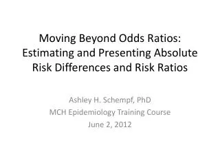
Moving Beyond Odds Ratios: Estimating and Presenting Absolute Risk Differences and Risk Ratios. Ashley H. Schempf, PhD MCH Epidemiology Training Course June 2, 2012. Acknowledgements. Jay Kaufman, PhD McGill University Presentation at 17 th Annual MCH Epidemiology Conference

E N D
Moving Beyond Odds Ratios: Estimating and Presenting Absolute Risk Differences and Risk Ratios Ashley H. Schempf, PhD MCH Epidemiology Training Course June 2, 2012
Acknowledgements Jay Kaufman, PhD McGill University Presentation at 17th Annual MCH Epidemiology Conference New Orleans, LA 12/14/11 Kaufman & Schempf. “Absolute Epidemiology: Developing Software Skills for Estimation of Absolute Contrasts from Regression Models for Improved Communication and Greater Public Health Impact.”
Outline • Problems of the Odds Ratio • Not intuitive • Exaggerates risk, especially for common outcomes • Not collapsible over strata, apparent confounding • Why did we ever use it? Is it appropriate? • Absolute epidemiology • Actual risk and numbers affected (AR, PAR, NNT) • Additive interactions • How to calculate RD and RRs in SAS and STATA
Odds are….odd • We tend to think in probabilities • 3 out of 4, p=75% • Odds divide the probability by 1-p • 3 to 1 or p/(1-p)=0.75/0.25 = 3 to 1 • What if outcome (p) is rare? • 1-p → 1 and p gets closer to p/(1-p) • 1 out of 10, p=10% • 1 to 9 or p/(1-p)=0.1/0.9 = 0.11 to 1
Risks versus Odds Davies HT, Crombie IK, Tavakoli M. When can odds ratios mislead? BMJ. 1998 Mar 28;316(7136):989-91.
Oddness of Odds Ratios • Compare the outcomes in two groups Odds in Group 2: P2/(1-P2) Odds in Group 1: P1/(1-P1) • Correct Interpretation: Group 2 has (1-OR)% increased odds of outcome Y compared to Group 1 • Problem: temptation to interpret as relative risks because a ratio of odds is difficult to understand; OR does not approximate RR when outcome is common = OR
OR versus RR • RR = P2/P1 • OR = RR* • For RRs>1, a doubling can occur • When P1 is small and P2 is much greater • For p1=.1, p2=(.1+1)/2=.55 ; RR=5.5; OR=11 • As P1 increases, the distance to P2 doesn’t have to be as large • For p1=.5, p2=(.5+1)/2=0.75; RR=1.5; OR=3
ORs will be exaggerated measures of RR • At high prevalence levels, regardless of RR • Even at low prevalence levels when RR is high • So basically, when prevalence is high in at least one strata
Case Example • Many public health problems are not very rare • Diabetes, Hypertension, Obesity • RR = .50/.35 = 1.43 • OR = (0.50/0.50)/(0.35/0.65) = 1.86
Non-collapsability • Unlike the RR, the odds ratio is not collapsible, meaning that the overall odds ratio does not equal the weighted average of stratum-specific odds ratios • The overall OR is always less so it can appear that there is significant confounding when there is none
The observed values are: Crude RR = 6/4 = 1.50 Crude OR = (6/4)/(4/6) = 2.25 Greatly exaggerated because overall risk is high (~50%) Z cannot be a confounder of X because it is not associated with X, all possible combinations of Z and X have 5 observations
The observed effect contrast measures are therefore: Adjusted RD = Crude RD Adjusted RD = Crude RD Adjusted OR ≠ Crude OR
The Odds Ratio is a LIAR Based on the practical criteria traditionally employed for detecting confounding (i.e., a change-in-estimate approach), the decision in this example would be to adjust for covariate Z when using the OR as the effect measure but not RR or RD. The discrepancy arises because inequality between the crude and adjusted OR does not necessarily imply causal confounding if the OR does not approximate the RR. The odds ratio is not collapsible, meaning that the average of the stratum-specific values does not necessarily equal the crude value, even in the absence of confounding. Thus, adjusting for factors that are not confounders can make associations appear stronger based on the OR (i.e. negative confounding) but will not affect the RD or RR. Also possible for crude to equal adjusted OR when confounding is present.
Why did we use odds ratios? • Some convenient properties • Symmetric, odds of Y = 1/(odds of not Y) • OR of exposure given outcome = OR of outcome given exposure • Didn’t have the tools and modeling options • Misconception that you cannot use RR in cross-sectional studies • Not true, it just becomes a prevalence rate ratio • Even in case-control studies, there are ways around an OR
What if you’ve published ORs? • Don’t fret; qualitative inference is still the same even if magnitude is off • If OR was positive and significant, RR will be too • If OR was negative and significant, RR will be too • Hopefully, you did not evaluate confounding, control for non-confounders, or interpret OR as increased risks • But now we have the tools to report what we want (risk/prevalence differences and ratios) • So, down with the odds ratio!
Are RRs all you need? • Unfortunately, all ratio-based measures can be misleading whether or not they’re based on odds or probabilities • Take, for example, a relative risk of 2 • A doubling of risk sounds dramatic • 1% to 2%, RR=2 but absolute increase is 1%, still very unlikely to have outcome Y • 30% to 60%, RR=2 but absolute increase is 30%, now more likely than not to have outcome Y
Absolute Epidemiology • Absolute risk/prevalence differences carry advantage of assessing actual impact • Potentially avertable or excess cases • Number needed to treat, PARF • Additive interactions • Some believe we should abandon ratio based measures of association altogether
Teaching Example Kaufman JS. Toward a more disproportionate epidemiology. Epidemiology 2010 Jan;21(1):1-2. • Department Chair wants to evaluate the effectiveness of instruction • Professor X conducts an RCT Treatment Group Control Group (n=30) (n=30) Passed 18 6 Failed 12 24 Total 30 30 Pass Rate tripled with instruction: 18/6 = 3
Teaching Example, cont. • The economy shifted and drove smarter students back to school as job opportunities were more limited (baseline pass rate increased) Treatment Group Control Group (n=30) (n=30) Passed 24 8 Failed 16 22 Total 30 30 Ratio measure of effectiveness controls for baseline changes RR = 24/8 = 3
Teaching Example, cont • Professor argues that it’s better to be rewarded based on absolute number of students who passed with the aid of instruction • Period 1: 18 – 6 = 12 • Period 2: 24 – 8 = 16 • However, this increased during the economy due to the talent of the student pool and not due to improvements in teaching effectiveness • Ratio measures help to control for baseline differences so that comparisons examine treatment effects rather than compositional differences
Teaching Example, cont. • No one can deny that in the first assessment, 12 more students passed as a result of instruction • Or that 18 more students passed as a result of instruction in the second assessment • But to compare teaching effectiveness across the two assessments requires an adjustment for baseline pass rates
Inconsistencies between Absolute and Relative Differences • When evaluating the effect of a single factor within one group or time period, there is qualitative concordance • A positive RD will correspond with RR>1 • A negative RD will correspond with RR<1 • However, indicators can be inconsistent when comparing the effect in two groups or time periods (interactions) • In teaching example, absolute measures differed over time while RR remained constant
Disparity Assessment Over Time:Decreasing Rates of a Negative Outcome Absolute Disparity Declines but Relative Disparity Increases Absolute Disparity (RD): 5 to 4 Relative Disparity (RR): 2 to 3
Disparity Assessment Over Time:Decreasing Rates of a Negative Outcome Optimal Disparity Reduction: Both Absolute and Relative Disparities ↓ Absolute Disparity (RD): 5 to 2 Relative Disparity (RR): 2 to 1.67 When rates are declining, a RR ↓ always corresponds to RD ↓
Disparity Assessment Over Time:Increasing Rates of a Positive Outcome Absolute Disparity Does Not Change and Relative Disparity ↓ Absolute Disparity (RD): 20 to 20 Relative Disparity (RR): 1.33 to 1.11
Disparity Assessment Over Time:Increasing Rates of a Positive Outcome Optimal Disparity Reduction: Both Absolute and Relative Disparities ↓ Absolute Disparity (RD): 20 to 10 Relative Disparity (RR): 1.33 to 1.13 When rates are increasing, a RD ↓ always corresponds to RR ↓
Healthy People • Decline in both absolute and relative differences is best evidence of progress in disparity elimination • Relative measures of disparity are primary indicator of progress because they adjust for changes in the level of the reference point over time • Relative measures also have advantage of adjusting for differences in reference point when comparisons are made across objectives Keppel KG, Pearcy JN, Klein RJ. Measuring progress in Healthy People 2010. Healthy People 2010 Stat Notes. 2004 Sep;(25):1-16.
÷ = ÷ = 33.0 – 4.2 = 28.8 per 100,000 population 11.6 – 1.3 = 10.3
Additive versus Multiplicative Interaction • Multiplicative interaction may be an extreme standard; cases where multiplicative interaction is not present but additive is with important public health implications Joint effects exhibit additive interaction: increase of 50 cases versus expected 30 Multiplicative interaction not present, 3*2=6, RR of 6 expected and observed Same as Teaching Example, but that was different assessments of the same factor—teaching effectiveness—that may have warranted a ratio measure to control for baseline differences over time
Why both absolute and relative measures matter • Absolute measures quantify actual risks and number affected • Necessary to evaluate/interpret the meaning of a given RR • Relative measures allow standardized comparisons across groups, time periods, indicators • Lack of correspondence creates controversy of which is “better” but they provide complementary information
Accurate Media Reporting • Starts with researchers presenting appropriate statistics and understanding their own data • Bad example – Schulman et al, NEJM 1999 • Good example – Chen et al, JAMA 2011
Disparities in Cardiac Catheterization • Odds Ratios were interpreted as Risk Ratios (large discrepancy due to common outcome) • Universal effects of race and sex were purported when the only difference was for Black women • No effect of sex among Whites • No effect of race among Men • Wide mischaracterization of results in the media
Alcohol Use and Breast Cancer • Appropriately interpreted as a 50% increase in breast cancer risk comparing 0 daily intake to 2+ drinks/day, translating to a 1.3% point increase in the incidence of breast cancer over 10 years • “while the increased risk found in this study is real, it is quite small. Women will need to weigh this slight increase in breast cancer risk with the beneficial effects alcohol is known to have on heart heath, said Dr. Wendy Chen, of Brigham and Women's Hospital in Boston. Any woman's decision will likely factor in her risk of either disease, Chen said.” MSNBC
Estimation Options for Risk Differences and Risk Ratios Showing code in STATA and SAS Examples with non-sampled and complex survey data
Model Options • Linear Probability Model • Generalized Linear Model (Binomial, Poisson) • Logistic Model (probability conversions)
Simple Data Example • Linked Birth Infant Death Data Set, 2004 • Data from several cities • Outcome: Preterm Birth (<37 weeks gestation) • Covariates: Marital status, race/ethnicity, maternal age • Example applies to cohort or cross-sectional data generally and population-level (non-sampled) or simple random samples
Tabular Risk Differences (STATA): • . csptbunmar, by(race) istandard rd • race | RD [95% CI] • -----------------+------------------------------ • NH WHITE | 0.0376 0.0251, 0.0501 • NH BLACK | 0.0394 0.0218, 0.0570 • HISPANIC | 0.0187 0.0091, 0.0283 • OTHER | 0.0174 -0.0061, 0.0408 • -----------------+------------------------------ • Crude | 0.0387 0.0324, 0.0451 • I. Standardized | 0.0281 0.0208, 0.0355 • But tabular approaches are limited: • Can only adjust for 1-2 categorical confounders • Difficult to handle continuous exposures/covariates • Difficult to handle clustered data, other extensions • So we need to take a regression-based approach…
SAS Tabular procfreq; table race*unmar*ptb/relriskriskdiffcmh; format race race.; run; Adjusted RR Type of Study Method Value 95% Confidence Limits Cohort Mantel-Haenszel1.2149 1.1588 1.2737
Linear Probability Model: Advantages: very easy to fit single uniform estimate of RD economists will love you Disadvantages: possible to get impossible estimates does not directly estimate RR biostatisticians will hate you Fit an OLS linear regression on the binary outcome variable: Pr(Y=1|X=x) = β0 + β1X Note: Homoskedasticity assumption cannot be met, since variance is a function of p. Therefore, use robust variance.
regress ptbunmarc.mager##c.mageri.race, vce(robust) cformat(%6.4f) Linear regression Number of obs = 47157 F( 6, 47150) = 66.28 Prob > F = 0.0000 R-squared = 0.0098 Root MSE = .35008 ------------------------------------------------------------------------------ | Robust ptb | Coef. Std. Err. t P>|t| [95% Conf. Interval] -------------+---------------------------------------------------------------- unmar | 0.0333 0.0038 8.82 0.000 0.0259 0.0407 mager | -0.0139 0.0022 -6.18 0.000 -0.0183 -0.0095 | c.mager#| c.mager | 0.0003 0.0000 7.14 0.000 0.0002 0.0004 | race | 2 | 0.0610 0.0052 11.82 0.000 0.0509 0.0712 3 | 0.0015 0.0038 0.39 0.698 -0.0060 0.0090 4 | -0.0046 0.0066 -0.70 0.482 -0.0174 0.0082 | _cons | 0.2696 0.0309 8.72 0.000 0.2090 0.3302 ------------------------------------------------------------------------------ Adjusted RD for marital status = 0.0333 (95% CI: 0.0259, 0.0407)
Can use a post-estimation command to see what the RD is relative to the PTB probability for married women (p=0.1249) Unmarried probability = 0.1249 + 0.0333 (unmarried beta) relative to married (divide by 0.1249) = 1 + 0.0333/0.1249 • ~27% increased risk of PTB compared to the overall probability among married women • - Crude proxy because there was no error incorporated for the probability among married women and it’s not adjusted for other factors in the model
procsurveyregorder=formatted; class race; modelptb = unmarmager mager2 race /clparmsolution; format race race.; run; Adjusted RD for marital status = 0.0333 (95% CI 0.0259 , 0.0407) Same results as in Stata
Testing an Additive Interaction Between UNMAR & RACE procsurveyregorder=formatted; classunmar race; modelptb = unmarmager mager2 race unmar*race /clparmsolution; sliceunmar*race / sliceby(race='b HISPANIC') diff; formatunmaryn. race race.; run; There is a significant additive interaction; the adverse effect of being unmarried is lower among Hispanic women relative to non-Hispanic White women
Additive Interaction Between UNMAR & RACE Effect of Being Unmarried Among non-Hispanic White Women (reference group) The Slice statement (or contrast/estimate) can combine coefficients to obtain the effect among Hispanic women (0.04748 – 0.02579 = 0.02159) So being unmarried increases the probability of PTB by 4.7% among non-Hispanic Whites versus 2.2% among Hispanics
2) Generalized Linear Model: Advantages: single uniform estimate biostatisticians will love you Disadvantages: can be difficult to fit still possible to get impossible values Fit a GLM with a binomial or Poisson distribution For RD: identity link For RR: log link g[Pr(Y=1|X=x)] = β0 + β1X Generally fit Poisson when binomial fails to converge, must use robust standard errors due to binary data Spiegelman D, Hertzmark E. Easy SAS calculations for risk or prevalence ratios and differences. Am J Epidemiol 2005 Aug 1;162(3):199-200.
glmptbunmarc.mager##c.mageri.race, fam(binomial) lin(identity) cformat(%6.4f) binregptbunmarc.mager##c.mageri.race, rd cformat(%6.4f) Generalized linear models No. of obs = 47157 Optimization : MQL Fisher scoring Residual df = 47150 (IRLSEIM) Scale parameter = 1 Deviance = 38557.57844 (1/df) Deviance = .8177641 Pearson = 47156.96255 (1/df) Pearson = 1.000148 Variance function: V(u) = u*(1-u) [Bernoulli] Link function : g(u) = u [Identity] BIC = -468834.8 ------------------------------------------------------------------------------ | EIM ptb | Risk Diff. Std. Err. z P>|z| [95% Conf. Interval] -------------+---------------------------------------------------------------- unmar | 0.0304 0.0037 8.29 0.000 0.0233 0.0376 mager | -0.0138 0.0022 -6.33 0.000 -0.0180 -0.0095 | c.mager#| c.mager | 0.0003 0.0000 7.19 0.000 0.0002 0.0004 | race | 2 | 0.0608 0.0051 11.84 0.000 0.0507 0.0709 3 | 0.0021 0.0038 0.55 0.581 -0.0053 0.0095 4 | -0.0034 0.0065 -0.53 0.599 -0.0162 0.0093 | _cons | 0.2722 0.0299 9.12 0.000 0.2137 0.3307 ------------------------------------------------------------------------------
glmptbunmarc.mager##c.mageri.race, fam(binomial) lin(log) eform binregptbunmarc.mager##c.mageri.race, rrcformat(%6.4f) Generalized linear models No. of obs = 47157 Optimization : MQL Fisher scoring Residual df = 47150 (IRLSEIM) Scale parameter = 1 Deviance = 38541.14486 (1/df) Deviance = .8174156 Pearson = 47198.70916 (1/df) Pearson = 1.001033 Variance function: V(u) = u*(1-u/1) [Binomial] Link function : g(u) = ln(u) [Log] BIC = -468851.2 ------------------------------------------------------------------------------ | EIM ptb | Risk Ratio Std. Err. z P>|z| [95% Conf. Interval] -------------+---------------------------------------------------------------- unmar | 1.2733 0.0336 9.16 0.000 1.2092 1.3408 mager | 0.9184 0.0118 -6.64 0.000 0.8957 0.9418 | c.mager#| c.mager | 1.0018 0.0002 7.90 0.000 1.0013 1.0022 | race | 2 | 1.4499 0.0459 11.72 0.000 1.3626 1.5428 3 | 1.0098 0.0295 0.33 0.739 0.9535 1.0694 4 | 0.9632 0.0498 -0.72 0.469 0.8703 1.0661 ------------------------------------------------------------------------------
Risk Difference, Identity Link procgenmoddescending; class race/order=formatted; modelptb = unmarmager mager2 race / dist=bin link=identity; format race race.; run; Adjusted RD for marital status = 0.0304 (95% CI 0.0233 , 0.0375)
Relative Risk, Log Link procgenmoddescending; class race/order=formatted; modelptb = unmarmager mager2 race / dist=bin link=log; estimate'RR unmar'unmar1 /exp; format race race.; run; Adjusted RR for marital status = 1.27 (95% CI 1.21, 1.34)