Chapter 2 Limits
Chapter 2 Limits. Section 1 The tangent and velocity problems. 1. 1.1 The tangent problem. ‘touching’. Definition The tangent line is the limit position of the secant line. 2. 3. Example 1 Find an equation of the tangent line to the parabola. Solution. 4.

Chapter 2 Limits
E N D
Presentation Transcript
Chapter 2 Limits Section 1 The tangent and velocity problems 1
1.1 The tangent problem ‘touching’ Definition The tangent line is the limit position of the secant line. 2
Example 1 Find an equation of the tangent line to the parabola Solution 4
1.1 The velocity problem Example 2 Suppose that a ball is dropped from the upper observation deck of the CN Tower in Toronto, 450m above the ground. Find the velocity of the ball after 5 seconds. Analysis Through experiments carried out four centuries ago, Galieo’s Law is expressed by the equation The difficulty in finding the velocity after 5s is that we are dealing with a single instant of time (t=5), so no time interval is involved. We can approximate the desired quantity by computing the average velocity over the brief time interval. 5
In the preceding section, we have seen that how the limit arise when we want to find the tangent to a curve and the velocity of an object. We now turn our attention to limits in general and numerical and graphical for computing them. 7
Section 2 The Limits 2.1 Definition We write and say ‘the limit of f(x), as x approaches a, equals L’. If we can make the values of f(x) arbitrarily close to L(as close to L As we like) by taking x to be sufficiently close to a (on either side of a) but not equal to a. Notice: 8
Example 2 Evaluate the value of The problem is that the calculator gave false value because a calculator has a definite digit becuuse of its memory. As t approaches 0, the values of the function seem to approach 0.16666666……and so we guess that 10
Example 3 Investigate The value of oscillate between 1 and -1 infinitely often as x approaches 0. Example 4 Find 11
2.2 One side limits We write and say the left-hand linit of f(x) as x approaches a (or the limit of f(x) as x approaches a from the left) is equal to L if we can make the values of f(x) arbitrarily close to L by taking x to be sufficiently close to a and x less than a. 12
Theorem Example 4 The graph of a function is given. Use it to state the values (if they exist) of the following. 13
2.3 Infinite limits Example 5 Find The values of f(x) can be made arbitrarily large by taking x close enough to 0. Thus the value of f(x) do not approach a fixed number, so 14
Defenition Let f be defined on both sides of a, expect possibly at a itsself. then means that the values of f(x) can be made arbitrarily large negative by taking x sufficiently close to a, but not equal to a. 15
2.4 Asymptote Denefition The line x=a is called a vertical asymptote of the curve y=f(x) if at one of the following statement is true 16
Example 6 Find Example 7 Find the vertical asymptotes of Analysis There are potential vertical asymptotes where 17
Section 3 Calculating limits using the limit laws Limit LawsSuppose that C is a constant and the limits exits. Then 18
Example 8 Use the Limit Laws and the gaphs of f and g to evaluate the following limits, if they exits. 19
Expand the Limit Laws Example 8 Evaluate the following limits and justify each step. Direct Substitution Property if f is a polynomial or a rational function and a is in the domain of f, then 20
TheoremIf when x is near a (except possibly at a) and the limit of f and g both exist as x approaches a, then 22
The Squueeze Theorem If when x is near a (except possibly at a) and 23
Section 4 Continuity Continuity means a curve is continuous and the process is one that take place gradually without interruption or abrupt change. The graph can be drawn without removing your pen frpm the paper. 25
Definition 1 A function fis continuous at a number a if Notice: the definition of continuity implicitly requires three things 26
Example 1 The following shows the graph of a function f. At which numbers is f discontinuous ? Why? 27
Example 2 Where are each of the following functions discontinuous? 28
Definition 2 A function f is continuous from the right at a number a, if f is continuous from the left at a number a,if Example 3 Where is the greatest integral function continuous from the right or from the left. 29
Definition 3 A function f is continuous on an interval if it is continuous at every number in the interval. Notice: if f is defined only on one side of an endpoint of the interval, we understand continuous at the endpoint to mean continuous from the right or continuous from the left. Example 4 Show that the function is continuous at interval [-1,1]. 30
Theorem 4 If f and g are continuous at a and c is a constant, then the following functions are also continuous at a: 1. f+g 2. f-g 3. cf 4. fg Definition 3 A function f is continuous on an interval if it is continuous at every number in the interval. • Theorem 5 • Any polynomial is continuous everywhere; that is, it is continuous • on R • (b) Any rational function is continuous whereever it is defined; that is, • it is continuous on its domain. 31
Fomulas 6 Theorem 7 The following types of functions are continuous at every number in their domains: polynomials rational functions root functions trigonometric functions Example 5 On what intervals is each function continuous? Example 6 Evaluate 32
Theorem 8 If f is continuous at b and Theorem 9 If g is continuous at a and f is continuous at g(a), then the composite function by is continuous at a. That means a continuous function of a continuous functions is continuous at a. 33
Theorem 10 The Intermediate Value Theorem Suppose f is continuous on the closed interval [a,b] and let N be any number between f(a) and f(b), where Then there exists a number c in (a,b) such that f(c)=N. The Intermediate Value Theorem states that a continuous function takes on every intermeadiate value between the function values f(a) and f(b) once or more than once. Notice: The theorem is not true in general for discontinuous function. 35
In geometric terms, it says that if any horizontal line y=N is given between y=f(b) and y=f(a), then the curve must intersect y=Nsomewhere. Deduction If y=f(x) is continuous on the closed interval [a,b] and f(a)f(b)<0 , then the equation f(x)=0 has at lestone root. 36
The use of the Intermeadiat Value Theorem Locate roots of equations Example 8 Show that there is a root of the equation between 1 and 2. In fact, we can locate a root more precisely by using the intermeadiat value theoreom again and again. The method is shorten the closed Interval. 37