Many random walks are faster than one
290 likes | 495 Vues
Many random walks are faster than one. Random walks. Random step: Move to an adjacent node chosen at random (and uniformly) Random walk: Take an infinite sequence of random steps Random walks are cool! Who needs applications?. Applications. Graph exploration

Many random walks are faster than one
E N D
Presentation Transcript
Random walks • Random step: • Move to an adjacent node chosen at random (and uniformly) • Random walk: • Take an infinite sequence of random steps • Random walks are cool! Who needs applications?
Applications • Graph exploration • Randomization avoids need to know topology • Randomization rules when the graph is changing or unknown • Tracking • Hunters and prey start on different nodes • Hunters must locate and track prey • Communication: devices send messages at random • Exhibits locality, simplicity, low-overhead, robustness • Becoming a popular approach to mobile devices • And querying, searching, routing, self-stabilization in wireless ad hoc, peer-to-peer, and distributed systems • Example: find the max node when the edges go up and down • Can’t use depth-first search: can’t backtrack over a missing edge
Latency is a problem • There are many measures of latency: • Hitting time: Expected time E(H) to visit a given node • Cover time: Expected time E(C) to visit all nodes • Mixing time: Expected time to reach the stationary distribution • A walks spends an v fraction of time at node v on average • After the mixing time, a walk is at node v with probability v
Our question Can multiple walks reduce the latency? Choose a node v in a graph.Start k random walks from node v. Can k walks cover the graph k times faster than 1 walk? Our answer: Many times yes, but not always.
Outline • First some fun: Calculate speed-ups for simple graphs • Clique (complete graph): linear speed-up • Barbell: exponential speed-up • Cycle: logarithmic speed-up • Then some answers: When is linear speed-up possible? • Simple formulation of our linear speed-up result • General formulations of our linear speed-up result • In terms of the ratio cover-time/hitting-time • In terms of mixing time • Conclusions and open problems
Computer science probability • Coin flipping • p is the probability a coin lands heads • 1/p is the expected waiting time until a coin lands heads • Markov inequality • Chernoff inequality • When = log(n) and = 4, this probability is very small! • If you expect log(n) samples to be bad, then with high probability fewer than 5log(n) really are bad
Calculating speed-ups for simple graphs Let’s calculate E(C1) and E(Ck) for the clique, the barbell, the cycle.
Clique hitting time: n • A random walk starting at node A • Chooses a random node each step • Chooses node B with probability 1/n • Expected waiting time until choosing B is n • Hitting time from A to B is n B A
Clique cover time: n log(n) • Random walk visits nodes a1, a2, …, an • Assume i visited nodes, n-i unvisited nodes • (n-i)/n is probability the next node chosen is unvisited • n/(n-i) is the expected timed until an unvisted node is chosen • Cover time is a1 a2 … a3 … … ai … ai+1 … … an Ei = time to visit i+1st node after visiting ith node i nodes visited
Clique speed-up: k • A k-walk chooses nodes k times faster • 1 step of a k-walk chooses k nodes at random • k steps of a 1-walk chooses k nodes at random • Calculate expectations, then regroup terms:
Barbell cover time: n2 • The walk starts at O and moves to L or R: let’s say to L • The walk must move back to O in order to cover R • How long do we expect to wait for this L O transition? • From L, the walk moves to O with probability 1/(n+1) • Expect to fail n times and move to BL instead of O • From BL, the walk takes a long time to return to L • Remember the hitting time in the clique is n • Expect n steps to return to L from inside BL L O R BL BR (trust me)
Barbell speed-up: 2k • Start k=c log(n) walks on O (but let’s ignore ugly constants) • Expect half to move to BL, half to BR: that’s log(n) in each • Expect log(n) walks in BL and BR to stay there for n steps • Remember hitting time for the clique is n • Expect log(n) walks in BL and BR to cover them in n steps • Remember k-walk cover time for the clique is n log(n)/k • So expect log(n) walks to cover barbell in n steps, not n2 • Trust me: Proof must turn each “expect” into “with high probability” • Rejoice with me: That’s a speed up of n=2log(n) = 2k L O R BL BR
The cycle 0 1 n i+1 i-1 i
Cycle cover time: n2 0 1 n • Let Ei be expected time to reach 0 from i • E0 = 0 • Ei = 1 + Ei+1/2 + Ei-1/2 • En = E1 • Solve these recurrence relations • Show Ei = (i-1)E1 - (i-1)i • Notice Ei+1 – Ei = Ei – Ei-1 – 2 • Define Di+1 = Ei+1 – Ei and notice Di+1 = Di – 2 = E1 – 2i • Show E1 ≈ n • Notice E1 = En = (n-1)E1 - (n-1)n and solve for E1 • So Ei ≈ (i-1)n – (i-1)i = (i-1)(n-i) • Maximized at i = n/2 and maximum value is n2/4 i+1 i-1 i
Cycle speed-up: log(k) 0 1 n • Theorem: If Ck n2/s then s log k • Proof: We will show the following: n/2
Walk w takes n/2 more steps in one direction than the other • Let Si = +1 or -1 indicate whether w moves left or right at step i • Let Dt = S1 + S2 + + Stbe the difference in steps left – steps right • We can show using Chernoff • So
These speed-ups are all over the map! (linear, exponential, logarithmic) What is the right answer? When is linear speed-up possible? A simple answer. A general answer.
Matthews’ Theorem • Theorem: For any graph G C1 H1 log (n) • This bound may or may not be tight • On a clique, the cover time is nlog(n) and hitting time is n • On a line, the cover time and hitting time are both n2
Matthews’ Theorem for k walks • Theorem: For any graph G and k log(n) Ck(e/k) H1 log (n) + noise • Think of a random walk of length eH1 as a trial • Starting from any node, either the walk hits v or it doesn’t • Bound the probability that log(n) trials fail • A walk hits v in H1 expected time (hitting time definition) • A walk of length eH1 fails to hit v with probability < 1/e (Markoff) • So log(n) walks of length eH1 fails with probability < (1/e)log n = 1/n • Obtain log(n) trials using k random walks • k walks of length (log n/k) eH1 amount to log n trials • So the k-walk cover time is (e/k) H1 log (n) + noise
Simple speed-up • Theorem: When Matthews’ bound is tight, we have linear speed up for k log(n) • Proof: • C1=H1 log (n) when Matthew’s bound is tight • Ck (e/k) H1 log (n) by previous result • Ck (e/k) C1 • Observations: • Matthews is tight for many important graphs: cliques, expanders, torus, hypercubes, d-dimensional grids, d-regular balanced trees, certain random graphs, etc. • We can prove a speed-up even when Matthews is not tight …
General speed-up • Speed-up in terms of cover-time/hitting-time ratio: • Theorem: If R(n) = E(C1)/E(H1) and k R(n)1-, then E(Ck) (1/k) E(C1) + noise • When Matthews is tight, R(n) = log(n) • Replaces that constant e with 1, but at cost of slightly smaller k • Speed-up in terms of mixing time: • Theorem: If G is a d-regular graph with mixing time M, then E(Ck) (M log(n)/k) E(C1) + noise
Expanders • Expanders are highly-connected, sparse graphs: • Every nodes has degree d • Every set of at least half the nodes has at least n neighbors • Expanders have many applications: • Robust communication networks • Error correcting codes, random number generators, cryptography • Distributed memories, sorting networks, topology, physics… • Expanders yield impressive cover time speed-ups: • We proved linear speed-up for many graphs for k log n • We can prove linear speed-up for expanders for k n!
Conclusions • Linear speed-ups are possible for many important graphs • Speed-ups are related to the ratio C1/H1 of cover and hitting times • Linear speed-ups occur when this ratio is large • This result is tight… • Open problems: • Is the speed-up always at most k? always at least log k? • Is there a property characterizing speed-up better than C1/H1? • What if random walks start at different nodes, not the same node? • What is random walks can communicate or leave “breadcrumbs”? • What if the prey can move, not just the hunters? • What if the graph is actually changing dynamically?