Download
1 / 24
360 likes | 1.32k Vues
Transmission Line Theory. Introduction: In an electronic system, the delivery of power requires the connection of two wires between the source and the load. At low frequencies, power is considered to be delivered to the load through the wire.

E N D
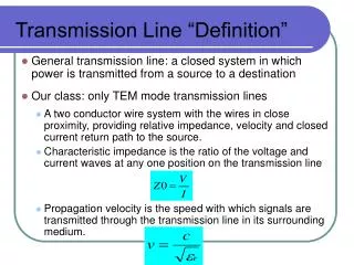
Transmission Line Theory Introduction: In an electronic system, the delivery of power requires the connection of two wires between the source and the load. At low frequencies, power is considered to be delivered to the load through the wire. In the microwave frequency region, power is considered to be in electric and magnetic fields that are guided from lace to place by some physical structure. Any physical structure that will guide an electromagnetic wave place to place is called a Transmission Line.
Types of Transmission Lines • Two wire line • Coaxial cable • Waveguide • Rectangular • Circular • Planar Transmission Lines • Strip line • Microstrip line • Slot line • Fin line • Coplanar Waveguide • Coplanar slot line
Analysis of differences between Low and High Frequency • At low frequencies, the circuit elements are lumped since voltage and current waves affect the entire circuit at the same time. • At microwave frequencies, such treatment of circuit elements is not possible since voltag and current waves do not affect the entire circuit at the same time. • The circuit must be broken down into unit sections within which the circuit elements are considered to be lumped. • This is because the dimensions of the circuit are comparable to the wavelength of the waves according to the formula: l = c/f where, c = velocity of light f = frequency of voltage/current
Transmission Line Concepts • The transmission line is divided into small units where the circuit elements can be lumped. • Assuming the resistance of the lines is zero, then the transmission line can be modeled as an LC ladder network with inductors in the series arms and the capacitors in the shunt arms. • The value of inductance and capacitance of each part determines the velocity of propagation of energy down the line. • Time taken for a wave to travel one unit length is equal to T(s) = (LC)0.5 • Velocity of the wave is equal to v (m/s) = 1/T • Impedance at any point is equal to Z = V (at any point)/I (at any point) Z = (L/C)0.5
Line terminated in its characteristic impedance: If the end of the transmission line is terminated in a resistor equal in value to the characteristic impedance of the line as calculated by the formula Z=(L/C)0.5 , then the voltage and current are compatible and no reflections occur. • Line terminated in a short: When the end of the transmission line is terminated in a short (RL = 0), the voltage at the short must be equal to the product of the current and the resistance. • Line terminated in an open: When the line is terminated in an open, the resistance between the open ends of the line must be infinite. Thus the current at the open end is zero.
Reflection from Resistive loads • When the resistive load termination is not equal to the characteristic impedance, part of the power is reflected back and the remainder is absorbed by the load. The amount of voltage reflected back is called voltage reflection coefficient. G = Vr/Vi where Vr = incident voltage Vi = reflected voltage • The reflection coefficient is also given by G = (ZL - ZO)/(ZL + ZO)
Standing Waves • A standing wave is formed by the addition of incident and reflected waves and has nodal points that remain stationary with time. • Voltage Standing Wave Ratio: VSWR = Vmax/Vmin • Voltage standing wave ratio expressed in decibels is called the Standing Wave Ratio: SWR (dB) = 20log10VSWR • The maximum impedance of the line is given by: Zmax = Vmax/Imin • The minimum impedance of the line is given by: Zmin = Vmin/Imax or alternatively: Zmin = Zo/VSWR • Relationship between VSWR and Reflection Coefficient: VSWR = (1 + |G|)/(1 - |G|) G = (VSWR – 1)/(VSWR + 1)
General Input Impedance Equation • Input impedance of a transmission line at a distance L from the load impedance ZL with a characteristic Zo is Zinput = Zo [(ZL + j Zo BL)/(Zo + j ZL BL)] where B is called phase constant or wavelength constant and is defined by the equation B = 2p/l
Half and Quarter wave transmission lines • The relationship of the input impedance at the input of the half-wave transmission line with its terminating impedance is got by letting L = l/2 in the impedance equation. Zinput = ZL W • The relationship of the input impedance at the input of the quarter-wave transmission line with its terminating impedance is got by letting L = l/2 in the impedance equation. Zinput = (Zinput Zoutput)0.5W
Effect of Lossy line on voltage and current waves • The effect of resistance in a transmission line is to continuously reduce the amplitude of both incident and reflected voltage and current waves. • Skin Effect: As frequency increases, depth of penetration into adjacent conductive surfaces decreases for boundary currents associated with electromagnetic waves. This results in the confinement of the voltage and current waves at the boundary of the transmission line, thus making the transmission more lossy. • The skin depth is given by: skin depth (m) = 1/(pmgf)0.5 where f = frequency, Hz m = permeability, H/m g = conductivity, S/m
Smith chart • For complex transmission line problems, the use of the formulae becomes increasingly difficult and inconvenient. An indispensable graphical method of solution is the use of Smith Chart.
Components of a Smith Chart • Horizontal line: The horizontal line running through the center of the Smith chart represents either the resistive ir the conductive component. Zero resistance or conductance is located on the left end and infinite resistance or conductance is located on the right end of the line. • Circles of constant resistance and conductance: Circles of constant resistance are drawn on the Smith chart tangent to the right-hand side of the chart and its intersection with the centerline. These circles of constant resistance are used to locate complex impedances and to assist in obtaining solutions to problems involving the Smith chart. • Lines of constant reactance: Lines of constant reactance are shown on the Smith chart with curves that start from a given reactance value on the outer circle and end at the right-hand side of the center line.
Solutions to Microwave problems using Smith chart • The types of problems for which Smith charts are used include the following: • Plotting a complex impedance on a Smith chart • Finding VSWR for a given load • Finding the admittance for a given impedance • Finding the input impedance of a transmission line terminated in a short or open. • Finding the input impedance at any distance from a load ZL. • Locating the first maximum and minimum from any load • Matching a transmission line to a load with a single series stub. • Matching a transmission line with a single parallel stub • Matching a transmission line to a load with two parallel stubs.
Plotting a Complex Impedance on a Smith Chart • To locate a complex impedance, Z = R+-jX or admittance Y = G +- jB on a Smith chart, normalize the real and imaginary part of the complex impedance. Locating the value of the normalized real term on the horizontal line scale locates the resistance circle. Locating the normalized value of the imaginary term on the outer circle locates the curve of constant reactance. The intersection of the circle and the curve locates the complex impedance on the Smith chart.
Finding the VSWR for a given load • Normalize the load and plot its location on the Smith chart. • Draw a circle with a radius equal to the distance between the 1.0 point and the location of the normalized load and the center of the Smith chart as the center. • The intersection of the right-hand side of the circle with the horizontal resistance line locates the value of the VSWR.
Finding the Input Impedance at any Distance from the Load • The load impedance is first normalized and is located on the Smith chart. • The VSWR circle is drawn for the load. • A line is drawn from the 1.0 point through the load to the outer wavelength scale. • To locate the input impedance on a Smith chart of the transmission line at any given distance from the load, advance in clockwise direction from the located point, a distance in wavelength equal to the distance to the new location on the transmission line.
Power Loss • Return Power Loss: When an electromagnetic wave travels down a transmission line and encounters a mismatched load or a discontinuity in the line, part of the incident power is reflected back down the line. The return loss is defined as: Preturn = 10 log10 Pi/Pr Preturn = 20 log10 1/G • Mismatch Power Loss: The term mismatch loss is used to describe the loss caused by the reflection due to a mismatched line. It is defined as Pmismatch = 10 log10 Pi/(Pi - Pr)
Microwave Components • Microwave components do the following functions: • Terminate the wave • Split the wave into paths • Control the direction of the wave • Switch power • Reduce power • Sample fixed amounts of power • Transmit or absorb fixed frequencies • Transmit power in one direction • Shift the phase of the wave • Detect and mix waves
Coaxial components • Connectors: Microwave coaxial connectors required to connect two coaxial lines are als called connector pairs (male and female). They must match the characteristic impedance of the attached lines and be designed to have minimum reflection coefficients and not radiate power through the connector. E.g. APC-3.5, BNC, SMA, SMC, Type N • Coaxial sections: Coaxial line sections slip inside each other while still making electrical contact. These sections are useful for matching loads and making slotted line measurements. Double and triple stub tuning configurations are available as coaxial stub tuning sections. • Attenuators: The function of an attenuator is to reduce the power of the signal through it by a fixed or adjustable amount. The different types of attenuators are: • Fixed attenuators • Step attenuators • Variable attenuators
Coaxial components (contd.) • Coaxial cavities: Coaxial cavities are concentric lines or coaxial lines with an air dielectric and closed ends. Propagation of EM waves is in TEM mode. • Coaxial wave meters: Wave meters use a cavity to allow the transmission or absorption of a wave at a frequency equal to the resonant frequency of the cavity. Coaxial cavities are used as wave meters.
Waveguide components • The waveguide components generally encountered are: • Directional couplers • Tee junctions • Attenuators • Impedance changing devices • Waveguide terminating devices • Slotted sections • Ferrite devices • Isolator switches • Circulators • Cavities • Wavemeters • Filters • Detectors • Mixers
Tees • Hybrid Tee junction: Tee junctions are used to split waves from one waveguide to two other waveguides. There are two ways of connecting the third arm to the waveguide – • along the long dimension, called E=plane Tee. • along the narrow dimension, called H-Plane Tee • Hybrid Tee junction: the E-plane and H-plane tees can be combined to form a hybrid tee junction called Magic Tee
Attenuators • Attenuators are components that reduce the amount of power a fixed amount, a variable amount or in a series of fixed steps from the input to the output of the device. They operate on the principle of interfering with the electric field or magnetic field or both. • Slide vane attenuators: They work on the principle that a resistive material placed in parallel with the E-lines of a field current will induce a current in the material that will result in I2R power loss. • Flap attenuator: A flap attenuator has a vane that is dropped into the waveguide through a slot in the top of the guide. The further the vane is inserted into the waveguide, the greater the attenuation. • Rotary vane attenuator: It is a precision waveguide attenuator in which attenuation follows a mathematical law. In this device, attenuation is independent on frequency.
Isolators • Mismatch or discontinuities cause energy to be reflected back down the line. Reflected energy is undesirable. Thus, to prevent reflected energy from reaching the source, isolators are used. • Faraday Rotational Isolator: It combines ferrite material to shift the phase of an electromagnetic wave in its vicinity and attenuation vanes to attenuate an electric field that is parallel to the resistive plane. • Resonant absorption isolator: A device that can be used for higher powers. It consists of a section of rectangular waveguide with ferrite material placed half way to the center of the waveguide, along the axis of the guide.