Download
1 / 26
260 likes | 387 Vues
Application of a hybrid EnKF-OI to ocean forecasting. Fran ç ois Counillon, Pavel Sakov, and Laurent Bertino. EnKF workshop 18 th June 2008. Project: NFR. Objectives. Two common approaches are often used: -Static ensemble: cheap computationally but uses static covariance

E N D
Application of a hybrid EnKF-OI to ocean forecasting François Counillon, Pavel Sakov, and Laurent Bertino EnKF workshop 18th June 2008 Project: NFR
Objectives • Two common approaches are often used: • -Static ensemble: cheap computationally but uses static covariance • -Dynamical ensemble: uses flow dependent covariance • but heavy computationally • In Counillon et al. (2008b), with 10 dynamical members ensemble in the Gulf of Mexico, the ensemble spread and the forecast error are correlated in space and time. • Hamill and Snyder (2000) and Wang et al. (2007) used both hybrid covariance for data assimilation. • Here, we apply small changes to the scheme, validate the advantage of the hybrid covariance for the EnKF and the ESRF and apply it to a realistic application of the Gulf of Mexico.
Outline • Methodology for data assimilation and hybrid covariance • Part I: • Validation of the EnKF-OI and ESRF-OI with a quasi-geostrophic model • Part II: • Demonstration of the EnKF-OI for a realistic application of the Gulf of Mexico
Static and dynamic approach Static methods (e.g. EnOI) Dynamical methods (e.g. EnKF, ESRF) Historical ensemble Dynamical ensemble Forecast Error Forecast Error Parameter introduced to rescale the variance of the static to the one of the forecast error
Hybrid approach We deduct a new ensemble matrix such as: • 3Dvar-EnKF Hamill and Snyder (2000) • ETKF-OI Wang et al. (2007) • But hybrid covariance used only for updating the ensemble mean • Here: • Hybrid covariance are used for updating the dynamical ensemble • Compare EnKF-OI vs. EnKF and ESRF-OI vs. ESRF • Test the method on a realistic application
Quasi-geostrophic model • Dimension (127*127), 1.5 layer reduced-gravity • Double-gyre wind forcing and biharmonic friction • Assimilation of 300 obs (2=4), every 10 time steps, rloc=25 grid cells
Experiment • Analyzing of the hybrid covariance for 5,10 .. 40 dynamical members • For a given size of dynamical ensemble, vary and (inflation) • Two schemes are used: EnKF, ESRF • Optimal values * and * are the ones that give a minimal error at the nowcast over 1000 model time steps Example for the ESRF-OI with 5 dynamical members
Conclusions (Part I) • Hybrid covariance methods provide better result than both static and dynamical methods. • Using the square root scheme improves and stabilizes the result • The method allows for a smooth transition between the: • EnOI, EnKF-OI, EnKF • EnOI, ESRF-OI, ESRF • The optimal linear blending coefficient * appears to decrease exponentially with the number of dynamical members, and is independent from the scheme used.
Realistic application of the ocean (part II) Gulf of Mexico: Strong velocity at the eddy fronts. Threat for off-shore industry Motivation for forecasting the position of the eddy fronts. Latex shelf West Florida Shelf Campeche Bank
Data assimilative system • Model presented in Counillon et al. (2008a) • TOPAZ3 (1/8o) gives lateral boundary condition to a high resolution model (1/22o) • Using HYCOM with 22 hybrid layers • Assimilation of altimetry maps • Forcing from ECMWF
Perturbation of the observation (spectral method, 50 km decorrelation radius) perturbs the position of the main features (LC, eddies) Perturbation of the lateral boundary condition (initial time lag) controls the position/growth of cyclonic eddies at the boundary of the LC Perturbation of the atmospheric forcing (spectral method, 50 km decorrelation radius) produces a uniformly small perturbation, and later on controls the position/growth of cyclonic eddies at the boundary of the LC Ensemble inflation (15%) improves slightly the accuracy Ensemble perturbation The perturbation system follows Counillon et al. (2008b)
Forecasting Error • Compare the EnOI with a 10 members EnKF and EnKF-OI • Used different values of beta for the EnKF-OI • Error computed for the 3 last runs (spin-up, shedding, data availability) • Calculate the daily RMSE, and interested in some questions: • Which is the optimal value of ? • Total average • Divergence ? • Run average • Stability with model propagation ? • Forecast horizon average • Where are the benefit located • Spatial average
Frontal analysisNowcast 12th July Background Ocean color, Black line SSH, pink spaghetti+redline EnKF-OI, yellow line EnOI
Frontal analysisNowcast 19th July Background Ocean color, Black line SSH, pink spaghetti+redline EnKF-OI, yellow line EnOI
Frontal analysisNowcast 26th July Background Ocean color, Black line SSH, pink spaghetti+redline EnKF-OI, yellow line EnOI
Ensemble variance Static EnKF-OI dyna 19th July
Correlation with SSHCenter of the GOM (point A) Analysis of the correlation a two target points Counillon et al. (2008a) Static Dyna 19th July hybrid Background correlation with SSH, white arrows, correlation with velocity
Correlation with SSHUpper shelf (point B) Static Dyna 19th July hybrid Background correlation with SSH, white arrows, correlation with velocity
Conclusion (Part II) • EnKF diverges with 10 members • EnKF-OI with 10 dynamical members reduces the forecast error by ~ 14 % compare to the EnOI at the nowcast • Gain from the EnOI increase with model propagation • Gain from the EnOI are mainly located on the fronts • In the correlation analysis, the benefits from the hybrid covariance are not large, but are stronger when the static approach fails
ConclusionAnalogy between the QG and the GOM experiment • The EnKF-OI can stabilize the EnKF, and provide more accurate result. • In the QG model *=0.6 whereas *=0.95 in GOM for 10 mem : • GOM model is of higher dimension • How would the hybrid covariance approach perform with highly non linear problem? • It is likely that assimilating track data in the GOM can bring further improvement • This might explain why the improvement from the EnOI are larger for the QG than for the GOM, at similar value of *
References • Counillon, F., P. Sakov, and L. Bertino, Application of a hybrid EnKF-OI to ocean forecasting, submitted to Ocean Dynamics , 2008c. • Counillon, F., and L. Bertino, Ensemble Optimal Interpolation: multivariate properties in the Gulf of Mexico, submitted to Tellus , 2008a. • Counillon, F., and L. Bertino, High resolution ensemble forecasting for the Gulf of Mexico eddies and fronts, submitted to Ocean Dynamics , 2008b. • Hamill, T., and C. Snyder, A Hybrid Ensemble Kalman Filterミ3D Variational Analysis Scheme, Monthly Weather Review , 128 , 2905ミ2919, 2000. • Wang, X., T. Hamill, J. Whitaker, and C. Bishop, A comparison of hybrid ensemble transform Kalman filter-OI and ensemble square-root filter analysis schemes, Mon. Wea. Rev , 2007.