EXPERIMENTAL ERRORS & STATISTICS
EXPERIMENTAL ERRORS & STATISTICS. SUHAILI ZAINAL ABIDIN FACULTY OF APPLIED SCIENCE UITM NEGERI SEMBILAN. The number of atoms in 12 g of carbon:. 602,200,000,000,000,000,000,000. The mass of a single carbon atom in grams:. 0.0000000000000000000000199. Scientific Notation. 6.022 x 10 23.

EXPERIMENTAL ERRORS & STATISTICS
E N D
Presentation Transcript
EXPERIMENTAL ERRORS & STATISTICS SUHAILI ZAINAL ABIDIN FACULTY OF APPLIED SCIENCE UITM NEGERI SEMBILAN
The number of atoms in 12 g of carbon: 602,200,000,000,000,000,000,000 The mass of a single carbon atom in grams: 0.0000000000000000000000199 Scientific Notation 6.022 x 10²³ 1.99 x 10-23 N x 10n N is a number between 1 and 10 n is a positive or negative integer Free powerpoint template: www.brainybetty.com
568.762 0.00000772 move decimal left move decimal right n > 0 n < 0 568.762 = 5.68762 x 10² 0.00000772 = 7.72 x 10⁻⁶ Addition or Subtraction • Write each quantity with the same exponent n • Combine N1 and N2 • The exponent,n, remains the same 4.31 x 10⁴ + 3.9 x 103 = 4.31 x 10⁴ + 0.39 x 104 = 4.70 x 10⁴ Free powerpoint template: www.brainybetty.com
Multiplication • Multiply N1 and N2 • Add exponents n1and n2 (4.0 x 10-5) x (7.0 x 103) = ? = (4.0 x 7.0) x (10-5+3) = 28 x 10-2 = 2.8 x 10⁻¹ (a x 10m) x (b x 10n) = (a x b) x 10m+n Division • Divide N1 and N2 • Subtract exponents n1and n2 8.5 x 10⁴÷ 5.0 x 109 = ? = (8.5 ÷ 5.0) x 104 - 9 = 1.7 x 10⁻⁵ (a x 10m) ÷ (b x 10n) = (a ÷b) x 10m-n Free powerpoint template: www.brainybetty.com
Significant Figures • - The meaningful digits in a measured or calculated quantity. • RULES: • Any digit that is not zero is significant • 1.234 kg 4significant figures • Zeros between nonzero digits are significant • 606 m 3 significant figures • Zeros to the left of the first nonzero digit are not significant • 0.08 L 1 significant figure • If a number is greater than 1, then all zeros to the right of the decimal point are significant • 2.0 mg 2 significant figures Free powerpoint template: www.brainybetty.com
If a number is less than 1, then only the zeros that are at the end and in the middle of the number are significant • 0.00420 g 3 significant figures • Numbers thatdo not contain decimal points, zeros after the last nonzero digit may or may not be significant. • 400 cm 1or 2 or 3 significant figures • 4 x 10² 1 significant figures • 4.0 x 10² 2 significant figures Free powerpoint template: www.brainybetty.com
How many significant figures are in each of the following measurements? 24 mL 2 significant figures 4 significant figures 3001 g 0.0320 m3 3 significant figures 6.4 x 10⁴ molecules 2 significant figures 560 kg 2 significant figures Free powerpoint template: www.brainybetty.com
89.332 + 1.1 one significant figure after decimal point two significant figures after decimal point 90.432 round off to 90.4 round off to 0.79 3.70 -2.9133 0.7867 Significant Figures Addition or Subtraction The answer cannot have more digits to the right of the decimal point than any of the original numbers. Free powerpoint template: www.brainybetty.com
3 sig figs round to 3 sig figs 2 sig figs round to 2 sig figs Significant Figures Multiplication or Division The number of significant figures in the result is set by the original number that has the smallest number of significant figures 4.51 x 3.6666 = 16.536366 = 16.5 6.8 ÷ 112.04 = 0.0606926 = 0.061 Free powerpoint template: www.brainybetty.com
QUESTION Free powerpoint template: www.brainybetty.com
LOGARITHMS AND ANTILOGARITHMS log 9.57 x 10-4 = -3.019 log 957 = 2.981 Example 3 2 Characteristics Mantissa 0.981 0.019 In converting a number to its logarithm, the number of digits in mantissa of the log of the number (957) should be equal to the number of SF in the number (957). For antilogarithm, 10 0.072 = 1.18 Free powerpoint template: www.brainybetty.com
Types of Errors in Chemical Analysis 1. Absolute Error Definition: The difference between the true value and the measured value E = xi – xt Where xi = measured value xt = true or accepted value Example: If 2.62 g sample of material is analyzed to be 2.52 g, so the absolute error is − 0.10g. Free powerpoint template: www.brainybetty.com
2. Relative Error Definition: The absolute or mean error expressed as a percentage of the true value. Er = xi – xt x 100% xt The above analysis has a relative error of − 0.10 gx 100% = -3.8% 2.62 g * We are usually dealing with relative errors of less than 1%. A 1% error is equivalent to 1 part in 100. Free powerpoint template: www.brainybetty.com
2.1 Relative Accuracy Definition: The measured value or mean expressed as a percentage of the true value. Er = xi x 100% xt The above analysis has a relative accuracy of 2.52 gx 100% = 96.2 % 2.62 g Free powerpoint template: www.brainybetty.com
3. Systematic Error or determinate error • Definition: A constant error that originates from a fixed cause, such as flaw in the design of an equipment or experiment. • It caused the mean of a set data to differ from the accepted value. • This error tends to cause the results to either high every time or low every time compared to the true value. • There are 3 types of systematic error: Oct 2008 Free powerpoint template: www.brainybetty.com
3.1 Instrumental Errors • All measuring devices contribute to systematic errors. • Glassware such as pipets, burets, and volumetric flasks may hold volume slightly different from those indicated by their graduations. • Occur due to significant difference in temperature from the calibration temperatere. • Sources of uncertainties: Decreased power supply voltage Increases resistance in circuits due to temperature change Free powerpoint template: www.brainybetty.com
3.2 Method Errors • Non-ideal analytical methods are often sources of systematic errors. • These errors are difficult to detect. • The most serious of the 3 types of systematic errors. Free powerpoint template: www.brainybetty.com
3.3 Personal Errors • Involve measurements that require personal judgment. • For example : • i) estimation of a pointer between tow scale divisions. • ii) color of solution. • iii) level of liquids with respect to a graduation in a burette. • iv) prejudice. Free powerpoint template: www.brainybetty.com
3.4 Effect of Systematic Errors Free powerpoint template: www.brainybetty.com
3.5 Detection and Control of Systematic Errors Free powerpoint template: www.brainybetty.com
4 Random Error or Indeterminate error • Cause data to be scattered more or less symmetrically around a mean value. • It reflects the precision of the measurement. • This error is caused by the many uncontrollable variables in physical or chemical measurements. Free powerpoint template: www.brainybetty.com
5 Gross Error • Differ from indeterminate and determinate errors. • They usually occur only occasionally, may cause a result to be either high or low. • For example: • i) part of precipitate is lost before weighing, analytical results will be low. • ii) touching a weighing bottle with your fingers after empty mass will cause a high mass reading for a solid weighed. • Lead to outliers, results in replicate measurements that differs significantly from the rest of the results. Free powerpoint template: www.brainybetty.com
Errors in Chemical Analysis Impossible to eliminate errors. How reliable are our data? Data of unknown quality are useless! • Carry out replicate measurements • Analyse accurately known standards • Perform statistical tests on data
Defined as follows: • The average of the numbers • Add up all the numbers, then divide by how many numbers there are. Mean Where xi = individual values of x and N = number of replicate measurements Median The middle result when data are arranged in order of size (for even numbers the mean of middle two). Median can be preferred when there is an “outlier” - one reading very different from rest. Median less affected by outlier than is mean.
Illustration of “Mean” and “Median” Results of 6 determinations of the Fe(III) content of a solution, known to contain 20 ppm: Note: The mean value is 19.78 ppm (i.e. 19.8ppm) - the medianvalue is 19.7 ppm
Precision • Precision of a measurement system, also called reproducibility or repeatability, is the degree to which repeated measurements under unchanged conditions show the same results • Relates to reproducibility of results.. • How similar are values obtained in exactly the same way? Useful for measuring this: Deviation from the mean:
Accuracy • Measurement of agreement between experimental mean and • true value (which may not be known!). • Measures of accuracy: • Accuracy of a measurement system is the degree of closeness of measurements of a quantity to its actual (true) value Absolute error: E = xi - xt (wherext = true or accepted value) Relative error: (latter is more useful in practice)
Illustrating the difference between “accuracy” and “precision” Low accuracy, low precision Low accuracy, high precision High accuracy, high precision High accuracy, low precision
Some analytical data illustrating “accuracy” and “precision” Benzyl isothiourea hydrochloride Analyst 4: imprecise, inaccurate Analyst 3: precise, inaccurate Analyst 2: imprecise, accurate Analyst 1: precise, accurate Nicotinic acid
Sample Standard Deviation, s • Standard deviation is a widely used measurement of variability or diversity used in statistics and probability theory. It shows how much variation or "dispersion" there is from the "average" (mean, or expected / budgeted value). • The equation for s must be modified for small samples of data, i.e. small N Two differences cf. to equation for s: 1. Use sample mean instead of population mean. 2. Use degrees of freedom, N - 1, instead of N. Reason is that in working out the mean, the sum of the differences from the mean must be zero. If N - 1 values are known, the last value is defined. Thus only N - 1 degrees of freedom. For large values of N, used in calculating s, N and N - 1 are effectively equal.
Alternative Expression for s (suitable for calculators) Note: NEVERround off figures before the end of the calculation
Reproducibility of a method for determining the % of selenium in foods. 9 measurements were made on a single batch of brown rice. Standard Deviation of a Sample Sample Selenium content (mg/g) (xI) xi2 1 0.07 0.0049 2 0.07 0.0049 3 0.08 0.0064 4 0.07 0.0049 5 0.07 0.0049 6 0.08 0.0064 7 0.08 0.0064 8 0.09 0.0081 9 0.08 0.0064 Sxi = 0.69 Sxi2= 0.0533 Mean = Sxi/N= 0.077mg/g (Sxi)2/N = 0.4761/9 = 0.0529 Standard deviation: Coefficient of variance = 9.2% Concentration = 0.077 ± 0.007 mg/g
Standard Error of a Mean The standard deviation relates to the probable error in a single measurement. If we take a series of N measurements, the probable error of the mean is less than the probable error of any one measurement. The standard error of the mean, is defined as follows:
Pooled Data To achieve a value of s which is a good approximation to s, i.e. N 20, it is sometimes necessary to pool data from a number of sets of measurements (all taken in the same way). Suppose that there are t small sets of data, comprising N1, N2,….Nt measurements. The equation for the resultant sample standard deviation is: (Note: one degree of freedom is lost for each set of data)
Pooled Standard Deviation Analysis of 6 bottles of wine for residual sugar.
Two alternative methods for measuring the precision of a set of results: VARIANCE: This is the square of the standard deviation: COEFFICIENT OF VARIANCE (CV) (or RELATIVE STANDARD DEVIATION): Divide the standard deviation by the mean value and express as a percentage:
Define some terms: CONFIDENCE LIMITS Interval around the mean that probably contains m. CONFIDENCE INTERVAL The magnitude of the confidence limits CONFIDENCE LEVEL Fixes the level of probability that the mean is within the confidence limits First assume that the known s is a good approximation to s. Examples later.
Percentages of area under Gaussian curves between certain limits of z (= x - m/s) 50% of area lies between 0.67s 80% “ 1.29s 90% “ 1.64s 95% “ 1.96s 99% “ 2.58s What this means, for example, is that 80 times out of 100 the true mean will lie between 1.29s of any measurement we make. Thus, at a confidence level of 80%, the confidence limits are 1.29s. For a single measurement: CL for m = x zs (values of z on next overhead) For the sample mean of N measurements , the equivalent expression is:
Values of z for determining Confidence Limits Confidence level, % z 50 0.67 68 1.0 80 1.29 90 1.64 95 1.96 96 2.00 99 2.58 99.7 3.00 99.9 3.29 Note: these figures assume that an excellent approximation to the real standard deviation is known.
Confidence Limits when s is known Atomic absorption analysis for copper concentration in aircraft engine oil gave a value of 8.53 mg Cu/ml. Pooled results of many analyses showed s ®s = 0.32 mg Cu/ml. Calculate 90% and 99% confidence limits if the above result were based on (a) 1, (b) 4, (c) 16 measurements. (b) (a) (c)
If we have no information on s, and only have a value for s - the confidence interval is larger, i.e. there is a greater uncertainty. Instead of z, it is necessary to use the parameter t, defined as follows: t = (x - m)/s i.e. just like z, but using s instead of s. By analogy we have: The calculated values of t are given on the next overhead
Values of t for various levels of probability Degrees of freedom 80% 90% 95% 99% (N-1) 1 3.08 6.31 12.7 63.7 2 1.89 2.92 4.30 9.92 3 1.64 2.35 3.18 5.84 4 1.53 2.13 2.78 4.60 5 1.48 2.02 2.57 4.03 6 1.44 1.94 2.45 3.71 7 1.42 1.90 2.36 3.50 8 1.40 1.86 2.31 3.36 9 1.38 1.83 2.26 3.25 19 1.33 1.73 2.10 2.88 59 1.30 1.67 2.00 2.66 1.29 1.64 1.96 2.58 Note: (1) As (N-1) , so t z (2) For all values of (N-1) < , t > z, I.e. greater uncertainty
Confidence Limits where s is not known Analysis of an insecticide gave the following values for % of the chemical lindane: 7.47, 6.98, 7.27. Calculate the CL for the mean value at the 90% confidence level. Sxi = 21.72 Sxi2 = 157.3742 If repeated analyses showed that s ® s = 0.28%:
Detection of Gross Errors A set of results may contain an outlying result - out of line with the others. Should it be retained or rejected? There is no universal criterion for deciding this. One rule that can give guidance is the Q test. The parameter Qexp is defined as follows:
Qexp is then compared to a set of values Qcrit: Qcrit (reject if Qexpt > Qcrit) No. of observations 90% 95% 99% confidencelevel 3 0.941 0.970 0.994 4 0.765 0.829 0.926 5 0.642 0.710 0.821 6 0.560 0.625 0.740 7 0.507 0.568 0.680 8 0.468 0.526 0.634 9 0.437 0.493 0.598 10 0.412 0.466 0.568 Rejection of outlier recommended if Qexp > Qcrit for the desired confidence level. Note:1. The higher the confidence level, the less likely is rejection to be recommended. 2. Rejection of outliers can have a marked effect on mean and standard deviation, esp. when there are only a few data points. Always try to obtain more data. 3. If outliers are to be retained, it is often better to report the median value rather than the mean.
Q Test for Rejection of Outliers The following values were obtained for the concentration of nitrite ions in a sample of river water: 0.403, 0.410, 0.401, 0.380 mg/l. Should the last reading be rejected? But Qcrit = 0.829 (at 95% level) for 4 values Therefore, Qexp < Qcrit, and we cannot reject the suspect value. Suppose 3 further measurements taken, giving total values of: 0.403, 0.410, 0.401, 0.380, 0.400, 0.413, 0.411 mg/l. Should 0.380 still be retained? But Qcrit = 0.568 (at 95% level) for 7 values Therefore, Qexp > Qcrit, and rejection of 0.380 is recommended. But note that 5 times in 100 it will be wrong to reject this suspect value! Also note that if 0.380 is retained, s = 0.011 mg/l, but if it is rejected, s = 0.0056 mg/l, i.e. precision appears to be twice as good, just by rejecting one value.
ANY QUESTIONS ?? Free powerpoint template: www.brainybetty.com
GOOD LUCK !! ~SUHAILI ZAINAL ABIDIN~ Free powerpoint template: www.brainybetty.com