Download
1 / 37
370 likes | 609 Vues
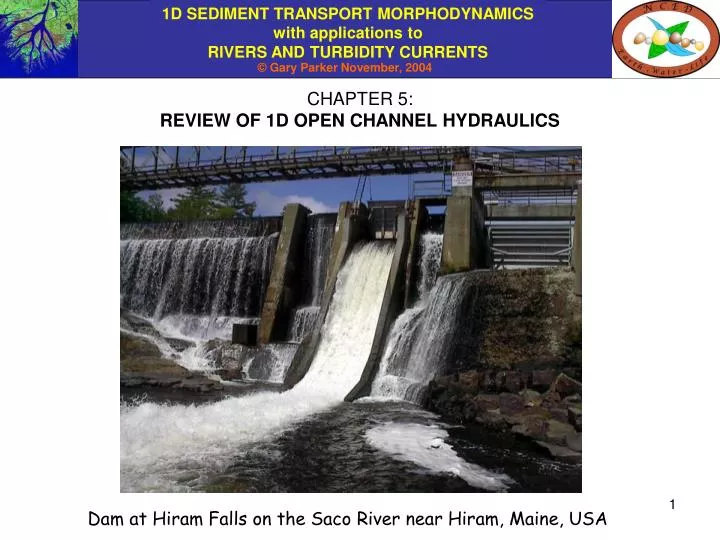
CHAPTER 5: REVIEW OF 1D OPEN CHANNEL HYDRAULICS. Dam at Hiram Falls on the Saco River near Hiram, Maine, USA. TOPICS REVIEWED.

E N D
CHAPTER 5: REVIEW OF 1D OPEN CHANNEL HYDRAULICS Dam at Hiram Falls on the Saco River near Hiram, Maine, USA
TOPICS REVIEWED • This e-book is not intended to include a full treatment of open channel flow. It is assumed that the reader has had a course in open channel flow, or has access to texts that cover the field. Nearly all undergraduate texts in fluid mechanics for civil engineers have sections on open channel flow (e.g. Crowe et al., 2001). Three texts that specifically focus on open channel flow are those by Henderson (1966), Chaudhry (1993) and Jain (2000). • Topics treated here include: • Relations for boundary resistance • Normal (steady, uniform) flow • St. Venant shallow water equations • Gradually varied flow • Froude number: subcritical, critical and supercritical flow • Classification of backwater curves • Numerical calculation of backwater curves
SIMPLIFICATION OF CHANNEL CROSS-SECTIONAL SHAPE River channel cross sections have complicated shapes. In a 1D analysis, it is appropriate to approximate the shape as a rectangle, so that B denotes channel width and H denotes channel depth (reflecting the cross-sectionally averaged depth of the actual cross-section). As was seen in Chapter 3, natural channels are generally wide in the sense that Hbf/Bbf << 1, where the subscript “bf” denotes “bankfull”. As a result the hydraulic radius Rh is usually approximated accurately by the average depth. In terms of a rectangular channel,
THE SHIELDS NUMBER: A KEY DIMENSIONLESS PARAMETER QUANTIFYING SEDIMENT MOBILITY b = boundary shear stress at the bed (= bed drag force acting on the flow per unit bed area) [M/L/T2] c = Coulomb coefficient of resistance of a granule on a granular bed [1] Recalling that R = (s/) – 1, the Shields Number * is defined as It can be interpreted as a ratio scaling the ratio impelling force of flow drag acting on a particle to the Coulomb force resisting motion acting on the same particle, so that The characterization of bed mobility thus requires a quantification of boundary shear stress at the bed.
QUANTIFICATION OF BOUNDARY SHEAR STRESS AT THE BED U = cross-sectionally averaged flow velocity ( depth-averaged flow velocity in the wide channels studied here) [L/T] u* = shear velocity [L/T] Cf = dimensionless bed resistance coefficient [1] Cz = dimensionless Chezy resistance coefficient [1]
RESISTANCE RELATIONS FOR HYDRAULICALLY ROUGH FLOW Keulegan (1938) formulation: where = 0.4 denotes the dimensionless Karman constant and ks = a roughness height characterizing the bumpiness of the bed [L]. Manning-Strickler formulation: where r is a dimensionless constant between 8 and 9. Parker (1991) suggested a value of r of 8.1 for gravel-bed streams. Roughness height over a flat bed (no bedforms): where Ds90 denotes the surface sediment size such that 90 percent of the surface material is finer, and nk is a dimensionless number between 1.5 and 3. For example, Kamphuis (1974) evaluated nk as equal to 2.
COMPARISION OF KEULEGAN AND MANNING-STRICKLER RELATIONS r = 8.1 Note that Cz does not vary strongly with depth. It is often approximated as a constant in broad-brush calculations.
BED RESISTANCE RELATION FOR MOBILE-BED FLUME EXPERIMENTS Sediment transport relations for rivers have traditionally been determined using a simplified analog: a straight, rectangular flume with smooth, vertical sidewalls. Meyer-Peter and Müller (1948) used two famous early data sets of flume data on sediment transport to determine their famous sediment transport relation (introduced later). These are a) a subset of the data of Gilbert (1914) collected at Berkeley, California (D50 = 3.17 mm, 4.94 mm and 7.01 mm) and the set due to Meyer-Peter et al. (1934) collected at E.T.H., Zurich, Switzerland (D50 = 5.21 mm and 28.65 mm). Bedforms such as dunes were present in many of the experiments in these two sets. In the case of 116 experiments of Gilbert and 52 experiments of Meyer-Peter et al., it was reported that no bedforms were present and that sediment was transported under flat-bed conditions. Wong (2003) used this data set to study bed resistance over a mobile bed without bedforms. Flume at Tsukuba University, Japan (flow turned off). Image courtesy H. Ikeda. Note that bedforms known as linguoid bars cover the bed.
BED RESISTANCE RELATION FOR MOBILE-BED FLUME EXPERIMENTS contd. Most laboratory flumes are not wide enough to prevent sidewall effects. Vanoni (1975), however, reports a method by which sidewall effects can be removed from the data. As a result, depth H is replaced by the hydraulic radius of the bed region Rb. (Not to worry, Rb H as H/B 0). Wong (2003) used this procedure to remove sidewall effects from the previously-mentioned data of Gilbert (1914) and Meyer-Peter et al. (1934). The material used in all the experiments in question was quite well-sorted. Wong (2003) estimated a value of D90 from the experiments using the given values of median size D50 and geometric standard deviation g, and the following relation for a log-normal grain size distribution; Wong then estimated ks as equal to 2D90 in accordance with the result of Kamphuis (1974), and s in the Manning-Strickler resistance relation as 8.1 in accordance with Parker (1991). The excellent agreement with the data is shown on the next page.
TEST OF RESISTANCE RELATION AGAINST MOBILE-BED DATA WITHOUT BEDFORMS FROM LABORATORY FLUMES
NORMAL FLOW Normal flow is an equilibrium state defined by a perfect balance between the downstream gravitational impelling force and resistive bed force. The resulting flow is constant in time and in the downstream, or x direction. • Parameters: • x = downstream coordinate [L] • H = flow depth [L] • U = flow velocity [L/T] • qw = water discharge per unit width [L2T-1] • B = width [L] • Qw = qwB = water discharge [L3/T] • g = acceleration of gravity [L/T2] • = bed angle [1] tb = bed boundary shear stress [M/L/T2] • S = tan = streamwise bed slope [1] • (cos 1; sin tan S) • = water density [M/L3] As can be seen from Chapter 3, the bed slope angle of the great majority of alluvial rivers is sufficiently small to allow the approximations
NORMAL FLOW contd. Conservation of water mass (= conservation of water volume as water can be treated as incompressible): Conservation of downstream momentum: Impelling force (downstream component of weight of water) = resistive force Reduce to obtain depth-slope product rule for normal flow:
ESTIMATED CHEZY RESISTANCE COEFFICIENTS FOR BANKFULL FLOW BASED ON NORMAL FLOW ASSUMPTION FOR u* The plot below is from Chapter 3
RELATION BETWEEN qw, S and H AT NORMAL EQUILIBRIUM Reduce the relation for momentum conservation b = gHS with the resistance form b = CfU2: Generalized Chezy velocity relation or Further eliminating U with the relation for water mass conservation qw = UH and solving for flow depth: Relation for Shields stress at normal equilibrium: (for sediment mobility calculations)
ESTIMATED SHIELDS NUMBERS FOR BANKFULL FLOW BASED ON NORMAL FLOW ASSUMPTION FOR b The plot below is from Chapter 3
RELATIONS AT NORMAL EQUILIBRIUM WITH MANNING-STRICKLER RESISTANCE FORMULATION Solve for H to find Solve for U to find Manning-Strickler velocity relation (n = Manning’s “n”) Relation for Shields stress at normal equilibrium: (for sediment mobility calculations)
BUT NOT ALL OPEN-CHANNEL FLOWS ARE AT OR CLOSE TO EQUILIBRIUM! And therefore the calculation of bed shear stress as b = gHS is not always accurate. In such cases it is necessary to compute the disquilibrium (e.g. gradually varied) flow and calculate the bed shear stress from the relation Flow over a free overfall (waterfall) usually takes the form of an M2 curve. Flow into standing water (lake or reservoir) usually takes the form of an M1 curve. A key dimensionless parameter describing the way in which open-channel flow can deviate from normal equilibrium is the Froude number Fr:
NON-STEADY, NON-UNIFORM 1D OPEN CHANNEL FLOWS: St. Venant Shallow Water Equations • x = boundary (bed) attached nearly horizontal coordinate [L] • y = upward normal coordinate [L] • = bed elevation [L] S = tan - /x [1] H = normal (nearly vertical) flow depth [L] Here “normal” means “perpendicular to the bed” and has nothing to do with normal flow in the sense of equilibrium. Bed and water surface slopes exaggerated below for clarity. Relation for water mass conservation (continuity): Relation for momentum conservation:
DERIVATION: EQUATION OF CONSERVATION OF OF WATER MASS Q = UHB = volume water discharge [L3/T] Q = Mass water discharge = UHB [M/T] /t(Mass in control volume) = Net mass inflow rate Reducing under assumption of constant B:
STREAMWISE MOMENTUM DISCHARGE Momentum flows! Qm = U2HB = streamwise discharge of streamwise momentum [ML/T2]. The derivation follows below. Momentum crossing left face in time Dt = (HBU2Dt) = mass x velocity Qm = momentum crossing per unit time, = (Momentum crossing in Dt)/ Dt = U2HB Note that the streamwise momentum discharge has the same units as force, and is often referred to as the streamwise inertial force.
STREAMWISE PRESSURE FORCE The flow is assumed to be gradually varying, i.e. the spatial scale Lx of variation in the streamwise direction satisfies the condition H/Lx << 1. Under this assumption the pressure p can be approximated as hydrostatic. Where z = an upward normal coordinate from the bed, p = pressure (normal stress) [M/L/T2] Integrate and evaluate the constant of integration under the condition of zero (gage) pressure at the water surface, where y = H, to get: Integrate the above relation over the cross-sectional area to find the streamwise pressure force Fp: Fp = pressure force [ML/T2]
DERIVATION: EQUATION OF CONSERVATION OF STREAMWISE MOMENTUM /t(Momentum in control volume) = net momentum inflow rate + sum of forces Sum of forces = downstream gravitational force – resistive force + pressure force at x – pressure force at x + x or reducing,
CASE OF STEADY, GRADUALLY VARIED FLOW Reduce equation of water mass conservation and integrate: constant Thus: Reduce equation of streamwise momentum conservation: But with water conservation: So that momentum conservation reduces to:
THE BACKWATER EQUATION Reduce with to get the backwater equation: where Here Fr denotes the Froude number of the flow and Sf denotes the friction slope. For steady flow over a fixed bed, bed slope S (which can be a function of x) and constant water discharge per unit width qw are specified, so that the backwater equation specified a first-order differential equation in H, requiring a specified value of H at some point as a boundary condition.
NORMAL AND CRITICAL DEPTH Consider the case of constant bed slope S. Setting the numerator of the right-hand side backwater equation = zero, so that S = Sf (friction slope equals bed slope) recovers the condition of normal equilibrium, at which normal depth Hn prevails: Setting the denominator of the right-hand side of the backwater equation = zero yields the condition of Froude-critical flow, at which Fr = 1 and depth = the critical value Hc: At any given point in a gradually varied flow the depth H may differ from both Hn and Hc. If Fr = qw/(gH3)1/2 < 1 the flow slow and deep and is termed subcritical; if on the other hand Fr > 1 the flow is swift and shallow and is termed supercritical. The great majority of flows in alluvial rivers are subcritical, but supercritical flows do occur. Supercritical flows are common during floods in steep bedrock rivers.
COMPUTATION OF BACKWATER CURVES The case of constant bed slope S is considered as an example. Let water discharge qw and bed slope S be given. In the case of constant bed friction coefficient Cf, let Cf be given. In the case of Cf specified by the Manning-Strickler relation, let r and ks be given. Compute Hc: Compute Hn: If Hn > Hc then (Fr)n < 1: normal flow is subcritical, defining a “mild” bed slope. If Hn < Hc then (Fr)n > 1: normal flow is supercritical, defining a “steep” bed slope. or where x1 is a starting point. Integrate upstream if the flow at the starting point is subcritical, and integrate downstream if it is supercritical. Requires 1 b.c. for unique solution:
COMPUTATION OF BACKWATER CURVES contd. Flow at a point relative to critical flow: note that It follows that 1 – Fr2(H) < 0 if H < Hc, and 1 – Fr2 > 0 if H > Hc. Flow at a point relative to normal flow: note that for the case of constant Cf and for the case of the Manning-Strickler relation It follows in either case that S – Sf(H) < 0 if H < Hn, and S – Sf(H) > 0 if H > Hn.
MILD BACKWATER CURVES M1, M2 AND M3 Again the case of constant bed slope S is considered. Recall that A bed slope is considered mild if Hn > Hc. This is the most common case in alluvial rivers. There are three possible cases. Depth increases downstream, decreases upstream M1: H1 > Hn > Hc Depth decreases downstream, increases upstream M2: Hn > H1 > Hc Depth increases downstream, decreases upstream M3: Hn > Hc > H1
M1 CURVE M1: H1 > Hn > Hc Water surface elevation = + H (remember H is measured normal to the bed, but is nearly vertical as long as S << 1). Note that Fr < 1 at x1: integrate upstream. Starting and normal (equilibrium) flows are subcritical. As H increases downstream, both Sf and Fr decrease toward 0. Far downstream, dH/dx = S d/dx = d/dx(H + ) = constant: ponded water As H decreases upstream, Sf approaches S while Fr remains < 1. Far upstream, normal flow is approached. The M1 curve describes subcritical flow into ponded water. Bed slope has been exaggerated for clarity.
M2 CURVE M1: Hn > H1 > Hc Note that Fr < 1 at x1; integrate upstream. Starting and normal (equilibrium) flows are subcritical. As H decreases downstream, both Sf and Fr increase, and Fr increases toward 1. At some point downstream, Fr = 1 and dH/dx = - : free overfall (waterfall). As H increases upstream, Sf approaches S while Fr remains < 1. Far upstream, normal flow is approached. The M2 curve describes subcritical flow over a free overfall. Bed slope has been exaggerated for clarity.
M3 CURVE M1: Hn > Hc > H1 Note that Fr > 1 at x1; integrate downstream. The starting flow is supercritical, but the equilibrium (normal) flow is subcritical, requiring an intervening hydraulic jump. As H increases downstream, both Sf and Fr decrease, and Fr decreases toward 1. At the point where Fr would equal 1, dH/dx would equal . Before this state is reached, however, the flow must undergo a hydraulicjump to subcritical flow. Subcritical flow can make the transition to supercritical flow without a hydraulic jump; supercritical flow cannot make the transition to subcritical flow without one. Hydraulic jumps are discussed in more detail in Chapter 23. The M3 curve describes supercritical flow from a sluice gate. Bed slope has been exaggerated for clarity.
flow subcritical supercritical HYDRAULIC JUMP In addition to M1, M2, and M3 curves, there is also the family of steep S1, S2 and S3 curves corresponding to the case for which Hc > Hn (normal flow is supercritical). These curves tend to be very short, and are not covered in detail here.
CALCULATION OF BACKWATER CURVES Here the case of subcritical flow is considered, so that the direction of integration is upstream. Let x1 be the starting point where H1 is given, and let x denote the step length, so that xn+1 = xn - x. (Note that xn+1 is upstream of xn.) Furthermore, denote the function [S-Sf(H)]/(1 – Fr2(H)] as F(H). In an Euler step scheme, or thus A better scheme is a predictor-corrector scheme, according to which A predictor-corrector scheme is used in the spreadsheet RTe-bookBackwater.xls. This spreadsheet is used in the calculations of the next few slides.
BACKWATER MEDIATES THE UPSTREAM EFFECT OF BASE LEVEL (ELEVATION OF STANDING WATER) A WORKED EXAMPLE (constant Cz): S = 0.00025 Cz = 22 qw = 5.7 m2/s D = 0.6 mm R = 1.65 H1 = 30 m H1 > Hn > Hc so M1 curve Example: calculate the variation in H and tb = CfU2in x upstream of x1 (here set equal to 0) until H is within 1 percent of Hn
RESULTS OF CALCULATION: PROFILES OF DEPTH H, BED SHEAR STRESS b AND FLOW VELOCITY U H tb U
RESULTS OF CALCULATION: PROFILES OF BED ELEVATION h AND WATER SURFACE ELEVATION x x h
REFERENCES FOR CHAPTER 5 Chaudhry, M. H., 1993, Open-Channel Flow, Prentice-Hall, Englewood Cliffs, 483 p. Crowe, C. T., Elger, D. F. and Robertson, J. A., 2001, Engineering Fluid Mechanics, John Wiley and sons, New York, 7th Edition, 714 p. Gilbert, G.K., 1914, Transportation of Debris by Running Water, Professional Paper 86, U.S. Geological Survey. Jain, S. C., 2000, Open-Channel Flow, John Wiley and Sons, New York, 344 p. Kamphuis, J. W., 1974, Determination of sand roughness for fixed beds, Journal of Hydraulic Research, 12(2): 193-202. Keulegan, G. H., 1938, Laws of turbulent flow in open channels, National Bureau of Standards Research Paper RP 1151, USA. Henderson, F. M., 1966, Open Channel Flow, Macmillan, New York, 522 p. Meyer-Peter, E., Favre, H. and Einstein, H.A., 1934, Neuere Versuchsresultate über den Geschiebetrieb, Schweizerische Bauzeitung, E.T.H., 103(13), Zurich, Switzerland. Meyer-Peter, E. and Müller, R., 1948, Formulas for Bed-Load Transport, Proceedings, 2nd Congress, International Association of Hydraulic Research, Stockholm: 39-64. Parker, G., 1991, Selective sorting and abrasion of river gravel. II: Applications, Journal of Hydraulic Engineering, 117(2): 150-171. Vanoni, V.A., 1975, Sedimentation Engineering, ASCE Manuals and Reports on Engineering Practice No. 54, American Society of Civil Engineers (ASCE), New York. Wong, M., 2003, Does the bedload equation of Meyer-Peter and Müller fit its own data?, Proceedings, 30th Congress, International Association of Hydraulic Research, Thessaloniki, J.F.K. Competition Volume: 73-80.