Download
1 / 54
540 likes | 750 Vues
Results from Three-Year WMAP Observations. Eiichiro Komatsu (UT Austin) TeV II Particle Astrophysics August 29, 2006. Why Care About WMAP?. WMAP observes CMB. This is a conference about “TeV” particle astrophysics. Why care about CMB?

E N D
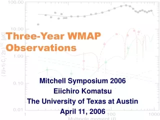
Results from Three-Year WMAP Observations Eiichiro Komatsu (UT Austin) TeV II Particle Astrophysics August 29, 2006
Why Care About WMAP? • WMAP observes CMB. This is a conference about “TeV” particle astrophysics. Why care about CMB? • The present-day temperature of CMB is 2.725K, or 2.35 meV. • The temperature at decoupling (where the most of CMB is coming from) was ~3000K, or 0.26 eV. • The temperature at matter-radiation equality was ~9000K, or 0.8 eV. • CMB is a nuisance for many particle astrophysicists: it attenuates cosmic-ray particles traveling through the universe. (GZK) • Why am I here?
What Can CMB Offer? • Baryon-to-photon ratio in the universe • Sound speed and inertia of baryon-photon fluid • Matter-to-radiation ratio in the universe • Dark matter abundance • “Radiation” may include photons, neutrinos as well as any other relativistic components. • Angular diameter distance to decoupling surface • Peak position in l space ~ (Sound horizon)/(Angular Diameter Distance) • Time dependence of gravitational potential • Integrated Sachs-Wolfe Effect, Dark energy • Primordial power spectrum (Scalar+Tensor) • Constraints on inflationary models • Optical depth • Cosmic reionization
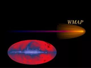
Full Sky Microwave Map COBE/FIRAS: T=2.725 K Uniform, “Fossil” Light from the Big Bang Cosmic Microwave Background Radiation
COBE/FIRAS, 1990 Perfect blackbody = Thermal equilibrium = Big Bang
COBE/DMR, 1992 Gravity is STRONGER in cold spots: DT/T~F
The Wilkinson Microwave Anisotropy Probe • A microwave satellite working at L2 • Five frequency bands • K (22GHz), Ka (33GHz), Q (41GHz), V (61GHz), W (94GHz) • The Key Feature: Differential Measurement • The technique inherited from COBE • 10 “Differencing Assemblies” (DAs) • K1, Ka1, Q1, Q2, V1, V2, W1, W2, W3, & W4, each consisting of two radiometers that are sensitive to orthogonal linear polarization modes. • Temperature anisotropy is measured by single difference. • Polarization anisotropy is measured by double difference.
The Angular Power Spectrum • CMB temperature anisotropy is very close to Gaussian; thus, its spherical harmonic transform, alm, is also Gaussian. • Since alm is Gaussian, the power spectrum: completely specifies statistical properties of CMB.
Physics of CMB Anisotropy • SOLVE GENERAL RELATIVISTIC BOLTZMANN EQUATIONS TO THE FIRST ORDER IN PERTURBATIONS
Use temperature fluctuations, Q=DT/T, instead off: Expand the Boltzmann equation to the first order in perturbations: where describes the Sachs-Wolfe effect: purely GR fluctuations.
For metric perturbations in the form of: Newtonian potential Curvature perturbations the Sachs-Wolfe terms are given by wheregis the directional cosine of photon propagations. • The 1st term = gravitational redshift • The 2nd term = integrated Sachs-Wolfe effect h00/2 (higher T) Dhij/2
Small-scale Anisotropy (<2 deg) • When coupling is strong, photons and baryons move together and behave as a perfect fluid. • When coupling becomes less strong, the photon-baryon fluid acquires shearviscosity. • So, the problem can be formulated as “hydrodynamics”. (c.f. The Sachs-Wolfe effect was pure GR.) Collision term describing coupling between photons and baryons via electron scattering.
Boltzmann Equation to Hydrodynamics • Multipole expansion • Energy density, Velocity, Stress Monopole: Energy density Dipole: Velocity Quadrupole: Stress
CONTINUITY EULER Photon-baryon coupling Photon Transport Equations f2=9/10 (no polarization), 3/4 (with polarization) FA = -h00/2, FH = hii/2 tC=Thomson scattering optical depth
Baryon Transport Cold Dark Matter
The Strong Coupling Regime SOUND WAVE!
The Wave Form Tells Us Cosmological Parameters Higher baryon density • Lower sound speed • Compress more • Higher peaks at compression phase (even peaks)
Ang.Diam. Distance ISW Baryon-to-photon Ratio Mat-to-Radiation Ratio What CMB Measures Amplitude of temperature fluctuations at a given scale, l~p/q 10 40 100 200 400 800 Multipole momentl~p/q Large scales Small scales
Measuring Matter-Radiation Ratio wheregis the directional cosine of photon propagations. • The 1st term = gravitational redshift • The 2nd term = integrated Sachs-Wolfe effect h00/2 (higher T) Dhij/2 During the radiation dominated epoch, even CDM fluctuations cannot grow (the expansion of the Universe is too fast); thus, dark matter potential gets shallower and shallower as the Universe expands --> potential decay --> ISW --> Boost Cl.
Matter-Radiation Ratio • More extra radiation component means that the equality happens later. • Since gravitational potential decays during the radiation era (free-fall time scale is longer than the expansion time scale during the radiation era), ISW effect increases anisotropy at around the Horizon size at the equality.
So, It’s Been Three Years Since The First Data Release. What Is New Now?
K Band (23 GHz) Dominated by synchrotron; Note that polarization direction is perpendicular to the magnetic field lines.
Ka Band (33 GHz) Synchrotron decreases as n-3.2 from K to Ka band.
Q Band (41 GHz) We still see significant polarized synchrotron in Q.
V Band (61 GHz) The polarized foreground emission is also smallest in V band. We can also see that noise is larger on the ecliptic plane.
W Band (94 GHz) While synchrotron is the smallest in W, polarized dust (hard to see by eyes) may contaminate in W band more than in V band.
Polarized Light Un-filtered Polarized Light Filtered
Seljak & Zaldarriaga (1997); Kamionkowski, Kosowsky, Stebbins (1997) Jargon: E-mode and B-mode • Polarization is a rank-2 tensor field. • One can decompose it into a divergence-like “E-mode” and a vorticity-like “B-mode”. E-mode B-mode
Physics of CMB Polarization • Thomson scattering generates polarization, if… • Temperature quadrupole exists around an electron • Where does quadrupole come from? • Quadrupole is generated by shear viscosity of photon-baryon fluid, which is generated by velocity gradient. electron isotropic no net polarization anisotropic net polarization
Boltzmann Equation • Temperature anisotropy, Q, can be generated by gravitational effect (noted as “SW” = Sachs-Wolfe) • Linear polarization (Q & U) is generated only by scattering (noted as “C” = Compton scattering). • Circular polarization (V) would not be generated. (Next slide.)
Primordial Gravity Waves • Gravity waves create quadrupolar temperature anisotropy -> Polarization • Directly generate polarization without kV. • Most importantly, GW creates B mode.
Power Spectrum Scalar T Tensor T Scalar E Tensor E Tensor B
Polarization From Reionization • CMB was emitted at z~1088. • Some fraction of CMB was re-scattered in a reionized universe. • The reionization redshift of ~11 would correspond to 365 million years after the Big-Bang. IONIZED z=1088, t~1 NEUTRAL First-star formation z~11, t~0.1 REIONIZED z=0
Measuring Optical Depth • Since polarization is generated by scattering, the amplitude is given by the number of scattering, or optical depth of Thomson scattering: which is related to the electron column number density as Ne =
Polarization from Reioniazation “Reionization Bump”
Masking Is Not Enough: Foreground Must Be Cleaned • Outside P06 • EE (solid) • BB (dashed) • Black lines • Theory EE • tau=0.09 • Theory BB • r=0.3 • Frequency = Geometric mean of two frequencies used to compute Cl Rough fit to BB FG in 60GHz
Clean FG • Only two-parameter fit! • Dramatic improvement in chi-squared. • The cleaned Q and V maps have the reduced chi-squared of ~1.02 per DOF=4534 (outside P06)
3-sigma detection of EE. The “Gold” multipoles: l=3,4,5,6. BB consistent with zero after FG removal.
Parameter Determination: First Year vs Three Years • The simplest LCDM model fits the data very well. • A power-law primordial power spectrum • Three relativistic neutrino species • Flat universe with cosmological constant • The maximum likelihood values very consistent • Matter density and sigma8 went down slightly
What Should WMAP Say About Flatness? Flatness, or very low Hubble’s constant? If H=30km/s/Mpc, a closed universe with Omega=1.3 w/o cosmological constant still fits the WMAP data.
Constraints on GW • Our ability to constrain the amplitude of gravity waves is still coming mostly from the temperature spectrum. • r<0.55 (95%) • The B-mode spectrum adds very little. • WMAP would have to integrate for at least 15 years to detect the B-mode spectrum from inflation.