Download
1 / 24
240 likes | 396 Vues
Towards the Calibration of the Nonlinear Ring Model at Diamond. R. Bartolini Diamond Light Source Ltd John Adams Institute, University of Oxford. Summary. Motivations Theory and tracking results Pinger experiments at Diamond Pinger calibration Spectral lines detection

E N D
Towards the Calibration of the Nonlinear Ring Model at Diamond R. Bartolini Diamond Light Source Ltd John Adams Institute, University of Oxford
Summary • Motivations • Theory and tracking results • Pinger experiments at Diamond • Pinger calibration • Spectral lines detection • Correction of nonlinear resonances • Conclusions: perspectives and limits
Comparison Real Lattice to Model Accelerator Model Accelerator • Closed Orbit Response Matrix (LOCO) • Detuning with amplitude (and with momentum) • Frequency Map Analysis • Apertures and Lifetime • Frequency Analysis of Betatron Motion (resonance driving terms)
Frequency Analysis of betatron motion Example: Spectral Lines for Diamond lattice (.2 mrad kick in both planes – tracking data) Spectral Lines detected with SUSSIX (NAFF algorithm) • e.g. in the horizontal plane: • (1, 0) 1.10 10–3horizontal tune • (0, 2) 1.04 10–6 Qx + 2 Qz • (–3, 0) 2.21 10–7 4 Qx • (–1, 2) 1.31 10–7 2 Qx + 2 Qz • (–2, 0) 9.90 10–8 3 Qx • (–1, 4) 2.08 10–8 2 Qx + 4 Qz
Spectral lines and nonlinear resonances J. Bengtsson (1988): CERN 88–04, (1988). J. Laskar’s work: Physica D 56, 253, (1992) R. Bartolini, F. Schmidt (1998), Part. Acc., 59, 93, (1998). R. Tomas, PhD Thesis (2003) • The main spectral lines appear at frequencies which are linear combinations of the betatron tunes; • Each resonance driving term fjklm contributes to the Fourier coefficient of a definite spectral line; to the lowest perturbative order there’s a one-to-one correspondence e.g the (3,0) resonance driving term f3000 excites the (-2,0) spectral line • The amplitude and phase of spectral lines (and driving terms) vary along the ring;
Frequency Analysis of Betatron Motion and Lattice Model Reconstruction (1)A possible Scheme (R. Bartolini, F.Schmidt PAC05) Accelerator Model Accelerator • tracking data at all BPMs • spectral lines from model (NAFF) • build a vector of Fourier coefficients • beam data at all BPMs • spectral lines from BPMs signals (NAFF) • build a vector of Fourier coefficients e.g. targeting more than one line Define the distance between the two vector of Fourier coefficients
Frequency Analysis of Betatron Motion and Lattice Model Reconstruction (2) Least Square Fit (SVD) of accelerator parameters θ to minimize the distance χ2of the two Fourier coefficients vectors • Compute the “Sensitivity Matrix” M • Use SVD to invert the matrix M • Get the fitted parameters MODEL → TRACKING → NAFF → Define the vector of Fourier Coefficients (amplitude and phase of spectral lines) Define the parameters to be fitted (i.e. sextupole gradients) SVD → CALIBRATED MODEL
Comparison with LOCO-type of machine modelling LOCO Closed Orbit Response Matrix from model fitting quadrupoles, etc Linear lattice correction/calibration Closed Orbit Response Matrix measured Spectral lines from model Nonlinear lattice correction/calibration fitting sextupoles Spectral Lines measured
Fitting sextupole gradients to correct the s-dependence of the amplitude of the spectral lines (0,2) machine with errors ideal machine machine with errors + sextupole fit + correction ideal machine (0,2) (-2,0) (-2,0) (-1,2) (-1,-2) (-1,2) (-1,-2) (-3,0) (-3,0) Given a machine with random sextupole errors, generating noisy spectral lines (black-left), the sextupole were fitted to reproduce the target vector (red-left) given by the ideal model. In this way we can correct the nonlinear model of the ring
Errors reconstruction from tracking data Blue dots are the originally assigned random errors Red dots are the reconstruction of the errors obtained from the sextupole fit The fit procedure involves many spectral lines and many SVD iterations A detail reconstruction of the machine model and its correction is possible on tracking data
Pingers Calibration The pingers deliver a half sine pulse of 3s (Trev = 1.87 s) Experiments were performed using a fill with 100 bunches (1/10 fill) and 25 mA, with slighlty positive chromaticity 0.5 Maximum H and V amplitude of the excited oscillation as a function of the kicker voltage shows a linear dependence after correction of the non linearity of the BPM X pos = H pinger current * 0.0096 Y pos = V pinger current * 0.0016
All BPMs have turn-by-turn capabilities • excite the beam diagonally • measure tbt data at all BPMs • colour plots of the FFT H BPM number QX = 0.22 H tune in H Qy = 0.36 V tune in V V All the other important lines are linear combination of the tunes Qx and Qy BPM number m Qx + n Qy frequency / revolution frequency
Linear lattice from turn-by-turn databeta functions The amplitude of the tune line is proportional to the square root of the beta function The beta functions at most BPMs are reproduced within few % except at the primary BPMs Bpm gains on primary are low by 10-15% (confirmed by LOCO) The linear optics was corrected with LOCO – coupling < 0.2% S (m)
Spectral line (-1, 1) in V associated with the sextupole resonance (-1,2) Comparison spectral line (-1,1) from tracking data and measured (-1,2) observed at all BPMs Spectral line (-1,1) from tracking data observed at all BPMs model model; measured BPM number BPM number
Spectral line (-2, 0) in H associated with the sextupole resonance (3,0) Comparison spectral line (-2,0) from tracking data and measured (-2,0) observed at all BPMs Spectral line (-2,0) from tracking data observed at all BPMs model model; measured BPM number BPM number
Spectral lines (-1,1) in V measured vs modela first fit of the sextupole gradient Blue model; red measured A first attempt to fit the spectral line (-1,1), determined by the resonance (-1,2), improved the agreement of the spectral line with the model However the lifetime was worse by 15% The fit produced non realistic large deviation in the sextupoles (>10%); The other spectral lines were spoiled BPM number
fit of (-1,1) in V (-1,1) (-2,0) sextupoles start iteration 1 iteration 2 resonance correction This resonance is increasing!
Simultaneous fit of (-2,0) in H and (1,-1) in V (-1,1) (-2,0) sextupoles start iteration 1 iteration 2 Both resonance driving terms are decreasing
Sextupole variation Now the sextupole variation is limited to < 5% Both resonances are controlled and the lifetime improved by 10%
Limits of the Frequency Analysis technique BPMs precision in turn by turn mode (+ gain, coupling and non-linearities) 10 m with ~10 mA very high precision required on turn-by-turn data (not clear yet is few tens of m is sufficient); Algorithm for the precise determination of the betatron tune lose effectiveness quickly with noisy data. R. Bartolini et al. Part. Acc. 55, 247, (1995) BPM gain and coupling can be corrected by LOCO, but nonlinearities remain (especially for diagonal kicks) Decoherence of excited betatron oscillation reduce the number of turns available Studies on oscillations of beam distribution shows that lines excited by resonance of order m+1 decohere m times faster than the tune lines. This decoherence factor m has to be applied to the data R. Tomas, PhD Thesis, (2003)
Non-#linearities of BPM readings The relation between BPMs reading and beam position is linear only in a reduced region around the BPM block centre PBPM
Effect of BPM nonlinearities on a simple harmonic signal (one frequency) Signal from betatron oscillations is x; BPM nonlinearity fit outputs: ax5 + bx3 + c Xmax = 5 mm the 3Qx and 5Qx lines appear due to X3 and x5 terms This will compromise the detection of high order lines, but not the ones due to sextupoles… The amplitude of the tune line is only slightly changed by the nonlinearities of the BPM
Conclusions Pinger magnets were installed on the diamond storage ring and are operational since end September 07 Characterisation of the non-linear beam motion is ongoing: a wealth of information can be obtained from the turn-by-turn data Correction strategies are under investigation with the ambitious aim to reconstruct a non-linear model of the ring Multiple Resonance correction and Improvement in Touschek lifetime was achieved Many thanks to P. Kuske, I. Martin, G. Rehm, J. Rowland, F. Schmidt