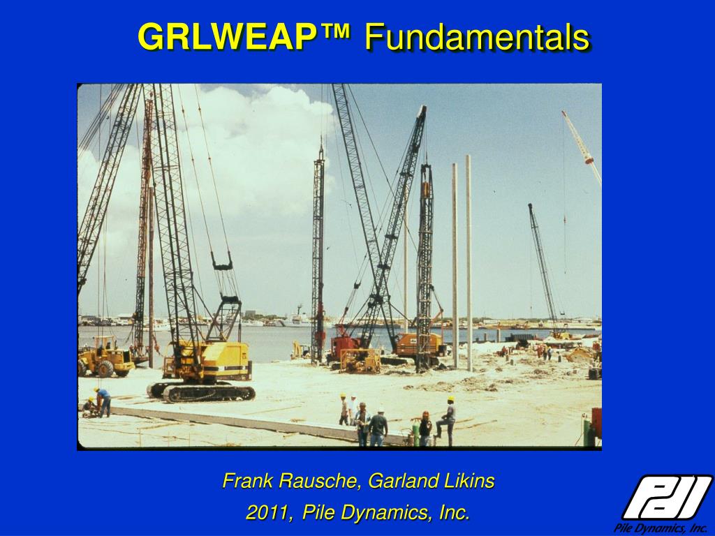
1. GRLWEAP™ Fundamentals Frank Rausche, Garland Likins 2011,Pile Dynamics, Inc.

2. CONTENT • Background and Terminology • Wave Equation Models • Hammer • Pile • Soil • The Program Flow • Bearing graph • Inspector’s Chart • Driveability

3. Some important developments in Dynamic Pile Analysis 1800s Closed Form Solutions & Energy Formulas 1950: Smith’s Wave Equation 1970: CAPWAP 1976: WEAP, TTI (mainframes) 1980s: GRLWEAP (PC’s) 1986: Hammer Performance Study 1996, 2006: FHWA Manual updates WEAP = Wave Equation Analysis of Piles

4. WAVE EQUATION OBJECTIVES • Smith’s Basic Premise: • Replace Energy Formula • Use improved pile model (elastic pile) • Use improved soil model (elasto-plastic static with damping) • Allow for stress calculations • Later GRLWEAP improvements: • realistic Diesel hammer model (thermodynamics) • comparison with pile top measurements • development of more reliable soil constants • driveability and inspectors’ chart options • residual stress analysis option

5. GRLWEAP Application • WHEN? • Before pile driving begins • After initial dynamic pile testing ( refined ) • WHY? • Equipment selection or qualification • Stress determination • Formulate driving criterion • Blow count calculation for desired capacity • Capacity determination from observed blow count

6. Some WEAP Terminology • Hammer Ram plus hammer assembly • Hammer assembly All non-striking hammer components • Hammer efficiency Ratio of Ek just before impact to Ep • Driving system All components between hammer and pile top • Helmet weight Weight of driving system • Hammer cushion Protects hammer - between helmet and ram • Pile cushion Protects pile - between helmet and pile top • Cap Generally the striker plate + hammer cushion+helmet • Pile damping Damping of pile material • Soil damping Damping of soil in pile-soil interface • Quake Pile displacement when static resistance reaches ultimate

7. Some WEAP Terminology • Bearing Graph Ult. Capacity and max. stress vs. blow count for a given penetration depth • Inspector’s Chart Calculates blow count and stresses for given ult. capacity at a given penetration depth as a function of stroke/energy • Driveability analysis Calculate blow count and stresses vs. depth based on static soils analysis • SRD Static Resistance to Driving • Soil set-up factor Ratio of long term to EOD resistance • Gain/loss factor Ratio of SRD to long term resistance • Variable set-up Setup occurring during a limited driving interruption

8. THE WAVE EQUATION MODEL • The Wave Equation Analysis calculates the movements (velocities and displacements) of any point of a slender elastic rod at any time. • The calculation is based on rod • Length • Cross Sectional Area • Elastic Modulus • Mass density

9. GRLWEAP Fundamentals • For a pile driving analysis, the “rod” is Hammer + Driving System + Pile • The rod is assumed to be elastic(?) and slender(?) • The soil is represented by resistance forces acting at the pile soil interface

10. GRLWEAP - 3 Hammer Models

11. External Combustion Hammer Modeling Cylinder and upper frame = assembly top mass Ram guides for assembly stiffness Drop height Ram: A, L for stiffness, mass Hammer base = assembly bottom mass

12. External Combustion HammersRam Model Ram segments ~1m long Combined Ram-H.Cushion Helmet mass

13. External Combustion HammersCombined Ram Assembly Model Ram segments Assembly segments Combined Ram-H.Cushion Helmet mass

14. Diesel Hammer Combustion Pressure Model • Compressive Stroke, hC • Cylinder Area, ACH • Final Chamber Volume, VCH • Max. Pressure, pMAX Precompression-Combustion-Expansion- pressures from thermodynamics Ports hC

15. DIESEL PRESSURE MODELLiquid Injection Hammers Pressure Port Closure Combustion Port Open Expansion Impact Compression pMAX Time

16. Program Flow – Diesel HammersFixed pressure, variable stroke Setup hammer, pile, soil model Downward = rated stroke Downward = upward stroke Next Ru? Calculate pile and ram motion N Strokes match? N Find upward stroke Output

17. Potential / Kinetic Energy WR WR h vi = Ö 2g h η EP = WR h (potential or rated energy) vi EK = ½ mR vi2 (kinetic energy) EK = ηEP (η - hammer efficiency) WP Max ET = ∫F(t) v(t) dt “Transferred Energy” EMX ETR = EMX/ ER = “transfer ratio”

18. GRLWEAP hammer efficiencies • The hammer efficiency reduces the impact velocity of the ram; reduction factor is based on experience • Hammer efficiencies cover all losses which cannot be calculated • Diesel hammer energy loss due to precompression or cushioning can be calculated and, therefore, is not covered by hammer efficiency

19. GRLWEAP diesel hammer efficiencies Open end diesel hammers: 0.80 (uncertainty of fall height, friction, alignment) Closed end diesel hammers: 0.80 (uncertainty of fall height, friction, power assist, alignment)

20. Other ECH efficiency recommendations Single acting Air/Steam hammers: 0.67 (fall height, preadmission, friction, alignment) Double acting Air/Steam/Hydraulic: 0.50 (preadmission, reduced pressure, friction, alignment) Drop hammers winch released: 0.50 (uncertainty of fall height, friction, and winch losses) Free released drop hammers (rare): 0.67 (uncertainty of fall height friction)

21. GRLWEAP hydraulic hammer efficiencies Hammers with internal monitor: 0.95 (uncertainty of hammer alignment) Hydraulic hammers (no monitor): 0.80 Power assisted hydraulic hammers: 0.80 (uncertainty of fall height, alignment, friction, power assist) If not measured, fall height must be assumed and can be quite variable – be cautious !

22. VIBRATORY HAMMER MODEL

23. VIBRATORY HAMMER MODEL Bias Mass with Line Force FL Connecting Pads m1 Oscillator with eccentric masses, me, radii, re and clamp m2 FV 2-mass system with vibratory force FV = me2 re sint FV = me [ω2resinωt - 2(t)]

24. GRLWEAP Hammer data file

25. Hammer: (Masses and Springs) Driving System: Cushions (Springs) Helmet (Mass) Hammer-Driving System-Pile-Soil Model Pile: Masses and Springs Soil: Elasto-Plastic Springs and Dashpots

26. Driving System Modeling The Driving Systems Consists of • Helmet including inserts to align hammer and pile • Hammer Cushion to protect hammer • Pile Cushion to protect concrete piles

27. GRLWEAP Driving System Help

28. GRLWEAP Driving System Help

29. GRLWEAP Pile Model To make realistic calculations possible • The pile is divided into N segments • of approximate length ∆L = 1 m (3.3 ft) • with mass m = ρ A ∆L • and stiffness k = E A / ∆L • there are N = L / ∆L pile segments • Divide time into intervals (typically 0.1 ms)

30. Computational Time Increment, ∆t Time ∆t is a fraction (e.g. ½ ) of the critical time, which is ∆L/c ∆tcr ∆L ∆t L/c Length

31. Driving system model (Concrete piles) Hammer Cushion: Spring plus Dashpot Helmet + Inserts Pile Cushion + Pile Top: Spring + Dashpot

32. Non-linear springsSprings at material interfaces Hammer interface springs Cushions Helmet/Pile Splices with slacks

33. Non-linear (cushion) springs • Parameters • Stiffness, k = EA/t • Coefficient of Restitution, COR • Round-out deformation,δr , or compressive slack • Tension slack, δs Compressive Force k /COR2 k Compressive Deformation δr δs

34. Hammer cushion Pile cushion

35. The Pile and Soil Model Mass density,  Modulus, E X-Area, A ∆L= L/N  1m Spring (static resistance) Dashpot (dynamic resist) Mass mi Stiffness ki

36. Soil Resistance • Soil resistance slows pile movement and causes pile rebound • A very slowly moving pile only encounters static resistance • A rapidly moving pile also encounters dynamic resistance • The static resistance to driving may differ from the soil resistance under static loads • Pore pressure effects • Lateral movements • Plugging for open profiles • Etc.

37. The Soil Model Segment i-1 Segment i Segment i+1 ki-1,Rui-1 Ji-1 ki,Rui RIGID SOIL SURROUNDING SOIL/PILE INTERFACE Ji ki+1,Rui+1 Ji+1

38. Smith’s Soil Model Segment i ui vi Total Soil Resistance Rtotal = Rsi +Rdi Fixed

39. Shaft Resistance and Quake Rsi -Rui Rui qi qi Recommended Shaft Quake ( qi ) 2.5 mm; 0.1 inches ui

40. Recommended Toe Quakes, qt R Rut qt qt u Non-displacement piles Displacement piles 0.1” or 2.5 mm 0.04” or 1 mm on hard rock D/120: very dense/hard soils D/60: softer/loose soils D

41. Smith’s Soil Damping Model (Shaft or Toe) Rd = RsJs v Pile Segment Smith damping factor, Js [s/m or s/ft] Fixed reference (soil around pile) Rd = RuJs v Smith-viscous damping factor Jsvi [s/m or s/ft] velocity v dashpot

42. Alternative Soil ModelsCoyle-Gibson Results (1968) Clay Sand

43. Recommended damping factorsafter Smith Shaft Clay: 0.65 s/m or 0.20 s/ft Sand: 0.16 s/m or 0.05 s/ft Silts: use an intermediate value Layered soils: use a weighted average Toe All soils: 0.50 s/m or 0.15 s/ft

44. Numerical treatment:Force balance at a segment Force from upper spring, Fi Acceleration: ai=(Fi – Fi+1+Wi– Ri) / mi Velocity, vi, and Displacement, ui, from Integration Mass mi Resistance force, Ri (static plus damping) Weight, Wi Force from lower spring, Fi+1

45. Wave Equation Analysis calculates displacement of all points of a pile as function of time. mi-1 Calculate displacements: uni = uoi + voit Calculate spring displacement: ci = uni - uni-1 Calculate spring forces: Fi = ki ci k = EA / ΔL uni-1 Fi, ci mi uni mi+1 uni+1

46. Set or Blow Count Calculation from Extrapolated toe displacement R Maximum Set Calculated Ru Extrapolated Set Final Set Quake

47. Blow Count Calculation • Once pile toe rebounds, max toe displacement is known, example: 0.3 inch or 7.5 mm • Final Set = Max Toe Displacement – Quake = 0.3 – 0.1 =0.2 inch = 7.5 - 2.5 = 5 mm • “Blow Count” is Inverse of “Final Set” BCT = 12 / 0.2 = 60 Bl / ft BCT = 1000 / 5 = 200 Bl / m

48. Alternative Blow Count Calculationby RSA • Residual Stress Analysis is also called Multiple Blow Analysis • Analyzes several blows consecutively with initial stresses, displacements from static state at end of previous blow • Yields residual stresses in pile at end of blow; generally lower blow counts

49. RESIDUAL STRESS OPTION BETWEEN HAMMER BLOWS, PILE AND SOIL STORE ENERGY Set for 2 Blows Convergence: Consecutive Blows have same pile compression/sets

50. COMPUTATIONAL PROCEDURESmith’s Bearing Graph • Analyze for a range of capacities • In: Static resistance distribution assumed • Out: Pile static capacity vs. blow count • Out: Critical driving stresses vs. blow count • Out: Stroke for diesel hammers vs. blow count