Artificial Life Lecture 13
360 likes | 531 Vues
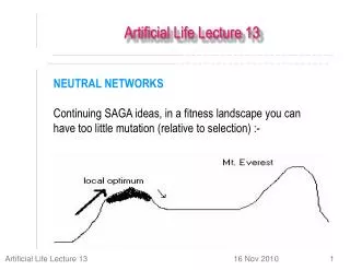
Artificial Life Lecture 13. NEUTRAL NETWORKS Continuing SAGA ideas, in a fitness landscape you can have too little mutation (relative to selection) :-. … or too much mutation. … or you can have too much mutation … (arrow up the hill is selection, arrow down the hill is mutation).

Artificial Life Lecture 13
E N D
Presentation Transcript
Artificial Life Lecture 13 NEUTRAL NETWORKS Continuing SAGA ideas, in a fitness landscape you can have too little mutation (relative to selection) :- Artificial Life Lecture 13
… or too much mutation … or you can have too much mutation … (arrow up the hill is selection, arrow down the hill is mutation) Artificial Life Lecture 13
… or just about the right amount … ... or you can gave round about the right amount, to avoid losing height (fitness) gained, but promoting search along ridges -- which may lead to higher ground :- Balance between exploration and exploitation Artificial Life Lecture 13
High dimensional landscapes We can visualise ridges in the 3-D landscapes (Himalayas, South Downs) that the metaphor of fitness landscapes draws upon. But in 100-D or 1000-D landscapes things can be very significantly different. In particular you can have ridges in all sorts of directions. Artificial Life Lecture 13
Ridges in high-dimensional landscapes Going from 2-D to 3-D allows extra opportunities for “bypasses around a valley without dropping height” Going up to 100-D or 1000-D potentially allows many many more such opportunities -- hyper-dimensional bypasses. (pic borrowed from Steps Towards Life, Manfred Eigen Oxford Univ Press 1992) Artificial Life Lecture 13
The First claim for Neutral Networks (1) The Formal claim It can be demonstrated indisputably thatIF a fitness landscape has lots of neutrality of a certain kind, giving rise to Neutral Networks with the property of constant innovation THEN the dynamics of evolution will be transformed (as compared to landscapes without neutrality) and in particular populations will not get stuck on local optima. The above would be merely a mathematical curiosity unless you can also accept:- Artificial Life Lecture 13
The Second claim for Neutral Networks (2) The Empirical claim Many difficult real design problems (..the more difficult the better...) in eg evolutionary robotics, evolvable hardware, drug design --- have fitness landscapes that naturally (ie without any special effort) fit the bill for (1) above. I make claim (2), but admit it is as yet a dodgy claim! Recently some supporting evidence. Artificial Life Lecture 13
Background to the Formal claim Most GA people would test their favourite GA on some benchmark fitness landscape, eg De Jong's test suite (Goldberg 1989, and other refs), or Kauffman's NK fitness landscape. It so happens that none of these benchmark tests have any neutrality, so not surprisingly they don’t notice any of the effects neutrality may bring. This has only been brought out by fairly recent research. Artificial Life Lecture 13
Recent Research on Neutral Networks One of the first demonstrations of the formal claim was in an EASy MSc dissertation by Lionel Barnett 1997. See full dissertation, and shorter version for Alife98 conference, on his web pages http://www.informatics.susx.ac.uk/users/lionelb/ and a (not-up-to-date) Neutral Network bibliography via http://www.informatics.susx.ac.uk/easy/ZOldWebsite/ResearchSeminars/NeutralNetworks_Bibliography.html Artificial Life Lecture 13
Tuneable Landscapes without Neutrality A good start-off place is with Kauffman's NK fitness landscape (not to be confused with Kauffman's NK Random Boolean Networks) See SA Kauffman The Origins of Order OUP 1993 or SA Kauffman At Home in the Universe pp 163 on Viking 1995 These give tuneable families of fitness landscapes without any neutrality. Artificial Life Lecture 13
The NK fitness landscape Binary genotypes of length N, with each gene epistatically linked to K others Each gene gives a 'fitness contribution' to the whole, depending on what its allele is (0 or 1) and on the alleles of its K neighbours. In the example above, K=2, and the fitness contribution of the marked gene depends on the 3 bits 100 There are 2(K+1) possible values of a gene and its K neighbours -- here for K=2 there are 23 = 8 possibilities. Artificial Life Lecture 13
0.385 0.129 0.975 0.010 0.398 0.603 0.427 0.220 000 001 010 011 100 101 110 111 Look-up tables There are 2(K+1) possible values of a gene and its K neighbours -- here for K=2 there are 23 = 8 possibilities. So, at this particular gene, we need a lookup table giving gene-fitness-contribution for each of the 8 possibilities -- here is a look-up table for this particular gene, where for a pattern 100 the contribution just happens to be 0.398 Artificial Life Lecture 13
Setting up an NK landscape (1) So, to set up a NK fitness landscape, you decide on N (length of gene) and K (epistatic nbrs), plus which are the specific epistatically-linked nbrs for each gene. For K=2 you would often count nbrs as those immediately Left and Right (with wrap-round at far left and far right) -- though one could specify different nbrhood relationships. You then generate N lookup tables of the appropriate size (2(K-1) entries), one separate one for each gene. Artificial Life Lecture 13
Setting up an NK landscape (2) You then fill in all the values in the lookup tables with random numbers uniformly drawn from range 0.0 to 1.0 So, the idea is: you specify only N and K, everything else is specified randomly. The fitness of any genotype of length N then comes from looking up the fitness-contribution of each gene, and adding them all together. This gives a generic tuneable fitness landscape -- with K=0 this is as smooth as you can get with K=N-1 this is as rugged as one can get Artificial Life Lecture 13
0.382 0.796 0 1 Smooth … For NK landscapes with K=0, each lookup table is tiny as here, options for 0 and 1 only So for each gene, there is a fitter value for that locus, independently of any other gene; here 1 is fitter than 0. So to maximise the sum of each gene-contribution, it is as simple as selecting the best value at each locus -- since there is here no epistatic linkage. This gives a really smooth Mt Fuji landscape. Artificial Life Lecture 13
… and Rugged As you increase K, landscapes get more rugged until at maximum K=N-1, any mutation at one locus will affect the fitness-contributions randomly from every locus -- maximum ruggedness, no correlation at all between fitnesses at neighbouring genotypes. Artificial Life Lecture 13
OK, now let’s add neutrality Work done in Lionel Barnett's EASy MSc project summer 1997 see http://www.informatics.susx.ac.uk/users/lionelb/ specially 'Ruggedness and Neutrality - the NKp family' Looked at adding Neutrality to the NK landscape, and analysing what difference it made to evolutionary dynamics. Adding neutrality = making sure there were lots of neutral ridges, ie mutations which made no change to the fitness. Artificial Life Lecture 13
NKp landscape NKp landscape -- fix N and K as before, create the lookup tables as before, and with probability p alter each lookup entry to exactly 0.0. Often p may be 0.95 or higher, ie 95% of entries are zero. Then a mutation at one locus will make changes in which entries are consulted in K+1 lookup tables -- and there is now a fair chance that in all cases the fitness-contribution changes from '0' to '0‘ -- ie does not change at all ! p is now an extra tuneable neutrality parameter. Artificial Life Lecture 13
The New Picture IF there is lots of neutrality of the right kind, then there are lots of Neutral Networks, connected pathways of neutral mutations running through the landscape at one level -- Artificial Life Lecture 13
… percolation … -- and lots and lots of these NNs, at different levels, percolating through the whole of genotype space, passing close to each other in many places. Without such neutrality, if you are stuck at a local optimum (ie no nbrs higher) then there are only N nbrs to look at BUT WHEN you have lots of neutrality, then without losing fitness you can move along a NN, with nearly N new nbrs at every step -- 'constant innovation'. Basically, you never get stuck ! Artificial Life Lecture 13
What happens? Roughly speaking, in such a landscape the population will quickly 'climb onto' a ridge slightly higher than average, then move around neutrally 'looking for a higher nbr to jump to'. You might have to wait a while (even a long while...) but you will not get stuck for ever. When eventually one of the popn finds a higher NN, the popn as a whole 'hops up‘ and carries on searching as before Artificial Life Lecture 13
Punk Eek ...and significantly, in many real GA problems this is just the sort of pattern that you see. The horizontal bits are not (as many thought) just standing still waiting for luck --- rather 'running along NNs waiting for luck' Artificial Life Lecture 13
Ruggedness versus Neutrality Lionel Barnett's NKp landscape gives an abstract framework in which one can tune independently: K for ruggedness and p for degree of Neutrality. There are various standard measures for ruggedness e.g. autocorrelation -- roughly, a measure of how closely related in height are points 1 apart, 2 apart, ...10 apart... Amazingly, for fixed N and K, when you tune parameter p all the way from zero neutrality up to maximum neutrality the autocorrelation remains (virtually) unchanged. Artificial Life Lecture 13
Same ruggedness but different dynamics Yet as you change the neutrality p, despite having the same ruggedness the evolutionary dynamics changes completely -- for zero neutrality the population gets easily stuck on local optima, for high neutrality it does not. Clearly neutrality makes a big difference -- yet this has been completely unknown to the GA community, who have only worried about ruggedness. Indeed all the typical benchmark problems used to compare different GAs have no neutrality at all. Artificial Life Lecture 13
Is this relevant to real problems? The formal claim has been proved. What about the empirical claim that neutrality exists (and is important) in many real problems? The Hand-wavy argument: Firstly, punk eek is seen in many evolutionary runs. Secondly, there are (for many real problems) far more different genotypes than there are different phenotypes. Eg in Adrian Thompson's hardware experiments, 21800 different genotypes but maybe 'only' 2600 or 21000 interestingly different phenotypes. Artificial Life Lecture 13
Verbal argument So for one specific phenotype (one fitness value) there may be 21200 or 2800 different genotypes that generate it. Colour all these dots red in genotype space -- a g.s. which is enormous but only 1800 steps across If these 21200 red dots are distributed at random, then they will not form connected paths or a network. BUT (...hand-waving..) it doesn’t require much underlying physical rationale to the genotype->phenotype mapping for there to be a tendency for red dots to cluster --> NNs ! Artificial Life Lecture 13
Empirical Evidence Firstly,(as before) punk eek is seen in many evolutionary runs. Secondly, NNs can be seen in plausible models of early RNA evolution (Schuster and colleagues) -- in fact this is where the ideas originated. Thirdly, relatively new work based on Adrian Thompson's hardware evolution experiments demonstrates conclusively (for the first time?) the existence of NNs in a non-toy problem. Artificial Life Lecture 13
NNs in Evolvable Hardware Evolvable hardware, genotypes of 1900 bits encode the wiring diagram of FPGA (rewireable silicon chips). 5 different chips, at different temperatures, are all wired up the same way, and all of them have to perform well at a tone-discrimination task. For this experiment, explicitly to check out whether NNs existed, effectively a popn of size 1 was used ! Variants on current one just had 3 mutations out of 1900 bits. Since maybe 2/3 was 'junk DNA', this is roughly equivalent to just a single effective mutation. Artificial Life Lecture 13
Results Results: typical 'punk eek' fitness graph, and we know that this is a pathway through genotype space in minimal steps. Let’s examine phenotypes (circuit wiring diagrams) A B C. Artificial Life Lecture 13
Phenotypic drift A and B have same fitness, yet genotypes and phenotypes have significant differences -- at different points along a NN. Artificial Life Lecture 13
Was the NN useful? B and C differ by a single mutation 'X', yet there is a fitness jump. IF you apply the same mutation 'X' to A, its fitness drops -- ie the drift from A to B was necessary. Artificial Life Lecture 13
A different example Vesselin Vassilev, evolving 3-bit multipliers (in terms of 2-input gates) – work presented at ICES2000 conference. Evolving an efficient 3-bit multiplier from scratch was tricky. So he started with the best known hand-designed one, and evolved neutrally (only functionally perfect ones accepted) with a bias towards more efficient ones. A ‘bridge’ through genotype space, 23% more efficient result. Artificial Life Lecture 13
Summary on NNs Neutral Networks is a hot new unexplored area. Origins in RNA evolution, Schuster and colleagues in Vienna. Still almost unknown -- apart from work done here at Sussex trying to make it relevant to applications, about the only non-RNA person who has spent time looking at this is Erik van Nimwegen at Santa Fe. Artificial Life Lecture 13
Implications for Applications Implications for applications: • You can expect in many circumstances (fingers crossed) there to be lots of NNs for free. • This means you neednt worry about getting stuck on local optima – needn’t worry about small popn sizes, which fits in with SAGA • Should worry about how to get the popn running around NNs searching as fast as possible, without 'falling off'. Artificial Life Lecture 13
Alife Projects Hand in proposals for feedback by Mon 22 Nov – and the following week’s seminars (Nov 30/ Dec 2) you are each asked to give a mini-presentation (2-4 minutes) on it:- • State your hypothesis (if scientific project) or end goal (if engineering), or … • What will be the criteria for success? • Give a rough overview of the methods you will use • Explain why these are reasonable methods for your aims • Cite 3 references from the existing literature that you will be using to guide your work Artificial Life Lecture 13
The End Time for Questions ?? Artificial Life Lecture 13