Download

1 / 16
220 likes | 592 Vues
Confidence Intervals for Two Proportions. Section 6.1. Section 6.1 CI for Two Proportions. We are interested in confidence intervals for the difference p 1 – p 2 between the unknown vlaues of two population proportions.

E N D
Confidence Intervals forTwo Proportions Section 6.1
Section 6.1CI for Two Proportions • We are interested in confidence intervals for the difference p1 – p2 between the unknown vlaues of two population proportions
6.1 Confidence Intervals for the difference p1 – p2 between two population proportions • In this section we deal with two populations whose data are qualitative. • For nominal data we compare the population proportions of the occurrence of a certain event. • Examples • Comparing the effectiveness of new drug versus older one • Comparing market share before and after advertising campaign • Comparing defective rates between two machines
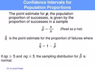
Parameter and Statistic • Parameter • When the data are qualitative, we can only count the occurrences of a certain event in the two populations, and calculate proportions. • The parameter we want to estimate is p1 – p2. • Statistic • An unbiased estimator of p1 – p2 is (the difference between the sample proportions).
x ˆ = p 1 1 n 1 Point Estimator: • Two random samples are drawn from two populations. • The number of successes in each sample is recorded. • The sample proportions are computed. Sample 1 Sample size n1 Number of successes x1 Sample proportion Sample 2 Sample size n2 Number of successes x2 Sample proportion
Large-sample CI for two proportions For two independent samples of sizes n1 and n2 with sample proportion of successes 1 and 2 respectively, an approximate level C confidence interval for p1 – p2is C is the area under the standard normal curve between −z* and z*. Use this method when
Icing the Kicker: 95% Confidence Interval Football coaches often employ the “icing the kicker” strategy. To ice the kicker the opposing coach calls for a timeout just before the kicker attempts a field goal, hoping that the delay interrupts the kicker’s concentration and causes him to miss the kick. Standard error of the difference p1−p2: 95% CI So the 95% CI is 0.024 ± 0.0672 = (0.0432, 0.0912) We are 95% confident that the interval 4.32% to 9.12% captures the true difference in the ABILITY of kickers to make a field goal when iced and their ABILITY to make a field goal when not iced. Because 0 is in the interval, we do not have convincing evidence that there is a significant difference in the ABILITY of kickers to make field goals when iced and when not iced.
Beware!! Common Mistake !!! A common mistake is to calculate a one-sample confidence interval for p1, a one-sample confidence interval for p2, and to then conclude that p1and p2 are equal if the confidence intervals overlap. This is WRONG because the variability in the sampling distribution for from two independent samples is more complex and must take into account variability coming from both samples. Hence the more complex formula for the standard error.
INCORRECT Two single-sample 95% confidence intervals: The confidence interval for the rightie BA and the confidence interval for the leftie BA overlap, suggesting no significant difference between Ryan Howard’s ABILITY to hit right-handed pitchers and his ABILITY to hit left-handed pitchers. Rightie interval: (0.274, 0.366) Leftie interval: (0.170, 0.280) 0 .095 .023 .167
Example: confidence interval for p1 – p2p. 2 • Estimating the cost of life saved • Two drugs are used to treat heart attack victims: • Streptokinase (available since 1959, costs $460) • t-PA (genetically engineered, costs $2900). • The maker of t-PA claims that its drug outperforms Streptokinase. • An experiment was conducted in 15 countries. • 20,500 patients were given t-PA • 20,500 patients were given Streptokinase • The number of deaths by heart attacks was recorded.
Example: confidence interval for p1 – p2(cont.) • Experiment results • A total of 1497 patients treated with Streptokinase died. • A total of 1292 patients treated with t-PA died. • Estimate the difference in the death rates when using Streptokinase and when using t-PA.
Example: confidence interval for p1 – p2(cont.) • Solution • The problem objective: Compare the outcomes of two treatments. • The data are nominal (a patient lived or died) • The parameter to be estimated is p1 – p2. • p1 = death rate with Streptokinase • p2 = death rate with t-PA
Example: confidence interval for p1 – p2(cont.) • Compute: Manually • Sample proportions: • The 95% confidence interval estimate is
Example: confidence interval for p1 – p2(cont.) • Interpretation • The interval (.0051, .0149) for p1 – p2 does not contain 0; it is entirely positive, which indicates that p1, the death rate for streptokinase, is greater than p2, the death rate for t-PA. • We estimate that the death rate for streptokinase is between .51% and 1.49% higher than the death rate for t-PA.
Example: 95% confidence interval for p1 – p2 The age at which a woman gives birth to her first child may be an important factor in the risk of later developing breast cancer. An international study conducted by WHO selected women with at least one birth and recorded if they had breast cancer or not and whether they had their first child before their 30th birthday or after. The parameter to be estimated is p1 – p2. p1 = cancer rate when age at 1st birth >30 p2 = cancer rate when age at 1st birth <=30 We estimate that the cancer rate when age at first birth > 30 is between .05 and .082 higher than when age <= 30.