Download
1 / 27
270 likes | 378 Vues
Explore numerical aspects of MO theory, variational theorem, and variational determination of MO's. Learn about the best wave function and its importance in quantum mechanics. Find out how to minimize energy expectation values to improve approximations systematically.

E N D
Lecture 26Molecular orbital theory II (c) So Hirata, Department of Chemistry, University of Illinois at Urbana-Champaign. This material has been developed and made available online by work supported jointly by University of Illinois, the National Science Foundation under Grant CHE-1118616 (CAREER), and the Camille & Henry Dreyfus Foundation, Inc. through the Camille Dreyfus Teacher-Scholar program. Any opinions, findings, and conclusions or recommendations expressed in this material are those of the author(s) and do not necessarily reflect the views of the sponsoring agencies.
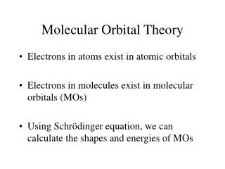
Numerical aspects of MO theory • We learn and carry out a mathematical procedure to determine the MO coefficients, which is based on variational theorem, Lagrange’s undetermined multiplier method, and matrix eigenvalue equation. • These are mathematical concepts of fundamental importance and their use and benefit go far beyond quantum chemistry.
What is the best wave function? • We have not discussed how to determine the expansion coefficients of LCAO MO’s (except when they are determined by symmetry). • To find the “best” LCAO MO’s with optimized coefficients, we must have a mathematical criterion by which to identify the “best” approximate wave function for a given Hamiltonian.
Variational theorem • A general mathematical technique applicable to many problems of chemistry, physics, and mathematics (an important tool for many-body problems complementary to perturbation theory). • We learn its application to quantum mechanics. • Question: we have Nnormalized wave functions that may or may not be the eigenfunctions of the Hamiltonian H. What is the bestwave function for the ground state?
Variationaltheorem • Answer: evaluate the expectation values of energy:and pick the one with the lowest expectation value. That is the bestwave function. Why? ΨA ΨB ΨC ΨD
Variationaltheorem • Any wave function can be expanded (exactly) as a linear combination of eigenfunctions of H (completeness). True ground state WF Orthonormality Ground state energy Normalization
Variationaltheorem • The closer the wave function is to the true ground-state one (which is measured by how close c0 is to unity), the lower the energy gets. Equality holds when and only when the wave function is the true wave function. • We can vary (hence the name variational theorem) a wave function’s shape (while maintaining normalization) to minimize its energy expectation value to systematically improve the approximation.
Variational determination of MO’s • The MO is a linear combination of two AO’s: • We find coefficients that minimize the energy (assuming real orbitals and coefficients), • Under the normalization condition.
Minimization • At a minimum of a function, its first derivative (gradient) must be zero (a necessary but not a sufficient condition).
Constrained minimization • Question: How can we incorporate this constraint during minimization (without it, E is not bounded from below and a minimum does not exist)? • Answer: Lagrange’s undetermined multiplier method.
Lagrange’s undetermined multiplier method • We need to minimize Eby varying cAand cB, • With the constraint that the wave function remains normalized, • Step 1: We write the constraint into a “... = 0” form:
Lagrange’s undetermined multiplier method • Step 2: We define a new quantity L(Lagrangian) to minimize, where we also introduce an additional parameter λ (undetermined multiplier) • Step 3: Minimize L by varying cA and cB as well as λ with no constraint:
Lagrange’s undetermined multiplier method The 3rd equation reduces to the constraint, which we must satisfy Once the 3rd equation (constraint) is satisfied, the 1st and 2nd equations reduce to minimization of E by varying cA and cB. Minimization of E wrt two parameters with one constraint is equivalent to minimization of L wrt three parameters
Lagrange’s undetermined multiplier as a buy-one-get-one-free Please minimize this function. Wait … let me add this constraint. Don’t worry – I only added zero.
Matrix eigenvalue equation Overlap integral Coulomb integral Resonance integral (negative)
Matrix eigenvalue equation • Use approximation S= 0 to simplify This matrix corresponds to 1 in arithmetic: a unit matrix Matrix acts on a vector and returns the same vector, apart from a constant factor λ
Matrix eigenvalue equation Operator eigenvalue equation Hamiltonian operator or matrix eigenfunction eigenvector eigenvalue Matrix eigenvalue equation
What is λ? • This correspondence suggests that λ (undetermined) actually represents energy! +) The left-hand side becomes The right-hand side becomes We find that in fact λ = E!
Lagrange’s undetermined multiplier • Many chemistry and physics problems are recast into constrained minimization or maximization. • Lagrange’s method can convert them into unconstrained minimization or maximization with slightly increased dimension. • The undetermined multiplier ends up in representing an important physical quantity.
Matrix eigenvalue equation • How do we solve this equation? • Observation: two equations for three unknowns (cA, cB, and E)– indeterminate? • The indeterminacy is removed by the normalization constraint.
Matrix eigenvalue equation If this matrix has an inverse, we invariably obtain a trivial, nonphysical solution:
Inverse matrix Definition of inverse Unit matrix We have verified that this is indeed the inverse
Inverse matrix determinant If the determinant is zero, the inverse does not exist
Inverse matrix Determinant is nonzero trivial nonphysical solution physical solution Determinant is zero
Summary • Variational theorem gives us a way to identify the best approximate wave function for the ground state; it is the one with the lowest energy expectation value. • Variational theorem therefore leads to minimization of expectation value with the constraint that the wave function is normalized. • Constrained minimization can be converted to unconstrained minimization with slightly higher dimension by Lagrange’s undetermined multiplier method. • With these, optimization of LCAO MO’s becomes a matrix eigenvalue equation.