Triangle mesh processing
Triangle mesh processing. Slides by Marc van Kreveld for DDM. Triangle mesh processing. Changing the locations of vertices (improvement) Reducing the number of vertices (downsampling, simplification) Increasing the number of vertices (upsampling)


Triangle mesh processing
E N D
Presentation Transcript
Triangle mesh processing Slides by Marc van Kreveld for DDM
Triangle mesh processing • Changing the locations of vertices (improvement) • Reducing the number of vertices (downsampling, simplification) • Increasing the number of vertices (upsampling) • Fixing up holes andother problems (repair) • Making levels of detail
Triangle mesh processing • Downsampling for efficient storage, rendering and transmission • try to preserve quality • Upsampling to ensure sufficiently small triangles when deformations are applied • try to improve quality
Euler operators vertex removal vertex insertion edge collapse vertex split halfedge collapse restricted vertex split
More operators edge split edge flip edge flip vertex relocate vertex relocate
Quality measures • What can we all measure to “represent” quality? • Euclidean distance between a mesh and a changed version • change in volume between the two meshes • change of normals between the two meshes • shape/size of the triangles of the two meshes • lengths of the edges of the two meshes • difference in convexity/concavity at the edges • angular deficit at the vertices: 2 – the sum of the angles of all triangles incident to a vertex (one angle per triangle)
Quality measures • Angular deficit: 2 – the sum of the angles of all triangles (facets) incident to a vertex (one angle per triangle/facet) /2 2/3 – /3 (and /2)
Quality measures for vertices • Suppose we remove a vertex v of a mesh, consider the mesh before removal to be correct, then the mesh after removal has some error • Then we can try to remove the vertex that induces the smallest error • in distance • in volume • in normals • We need to retriangulate the gap, also while minimizing error vertex removal
Quality measures for vertices • The number of triangulations of a convex polygon with k vertices is k (k+1) (k+2) … (2k–4) / (k–2)!value k 3 4 5 6 7# ways 1 2 5 14 42 • The number of triangulations of other polygons (gaps after removing a vertex from a polyhedron)is at most this large vertex removal ?
Approach for mesh simplification • Choose a relevant error measure • Choose operators to be tried • Choose a target mesh size or error • While target not reached: • For all operators and all places to apply it: • Compute (local) error measure before and after the operator • Keep the one with smallest loss • Apply the operator that induces the smallest error according to the chosen measure
Example: terrain simplification • Assume a planar triangulation is given where every vertex also has a height (z-coordinate) • Use vertical error as the measure • Use vertex removal as the operator, and always use the (planar) Delaunay triangulation to fill the gap
Terrain simplification • The vertical error is only caused in each shaded region • We need to compute the maximum vertical distance between two sets of triangles covering the same region • If a vertex has constant degree,then it takes O(1) time • If all vertices have constant degree,then it takes O(n) time overall to find the vertex whose removal causes the smallest error (mesh with n vertices)
Terrain simplification • Suppose we measure error only at the vertex?
Terrain simplification • One iteration takes O(n) time • E.g. halving the number of vertices takes O(n2) time • Efficiency improvement: note that in a next iteration, nearly all vertices will compute the same error;only vertices adjacent to the vertex just removed have a different error
Terrain simplification • We can keep all errors induced in a priority queue • One iteration is then: • Remove the lowest error removal from the priority queue • Delete it from the mesh and restore it to be Delaunay • For the neighbors of the removed vertex: • Remove them from the priority queue • Recompute the induced error • Insert in the priority queue • One iteration typically takes O(log n) time now, instead of O(n)
3D mesh simplification • For vertex removal and other operators on 3D meshes we must make sure that the operator does not cause self-intersections suppose we remove vertices on the backside of a boundary model of this spoon
3D mesh simplification • Some operators can be illegal because the resulting mesh would not be a 2-manifold (with or without boundary) anymore edge collapse not allowed
Making a mesh more uniform • A simple method to spread points evenly in a space: move every point to the center of its Voronoi cell, and iterate this a few times (recompute the Voronoi diagram after moving all points, and move again)
Making a mesh more uniform • This can be done on a triangle mesh in 3D too, but one should use the Voronoi diagram on the surface and not the 3D Voronoi diagram
Progressive meshes • Multi-scale representation by Hoppe (1996) • Designed to address: • mesh simplification (reduce number of vertices) • level-of-detail approximation (allow various resolutions) • progressive transmission (successively refine a coarse model when transmitting) • mesh compression (reduce storage) • selective refinement (allow different levels-of-detail in a single mesh, e.g. for view dependency)
Progressive meshes • Main idea of the progressive mesh (PM): store a coarse mesh plus the sequence of operations to get to the most accurate/detailed mesh M0 M1 Mn most coarse mesh mesh with one vertex more mesh with n vertices more (most accurate)
Progressive meshes • Meshes for computer graphics: typically, much more than just geometry is stored • discrete attributes (material, …) • numerical attributes (color, normal, coordinates for a texture, …) • Discrete attributes are stored with the triangles • Numerical attributes are stored with the corners of a mesh (corner: a vertex-triangle pair; each triangle has three corners) corner
Progressive meshes • A mesh M = (K, V, D, S) where • K is the connectivity information stored • V is the geometry (coordinates) stored • D is the set of discrete attributes stored with triangles • S is the set of numerical attributes stored with corners(Hoppe calls it scalar attributes rather than numerical,and sees color and normal each as three separate values)
Progressive meshes • To build a PM, start with the most detailed version and then incrementally apply edge collapse operations to get from Mn to M0 • To get a good quality PM, a good scheme for choosing the next edge collapse must be found edge collapse vertex split
Progressive meshes • In the edge collapse of {vs,vt}, the vertex vt disappears and so do the triangles {vs,vt, vl} and {vs,vt, vr} vt vr vr vl vl vs vs
Progressive meshes • The inverse vertex split is denoted vsplit(s, l, r, t, A), where A stores the coordinates of vs, vt, the attributes of the affected corners (all corners at vs and vt, and one corner at vl and vr), and the discrete attributes of the two appearing triangles vt vr vr vsplit vl vl vs vs
Progressive meshes • The PM representation is ( M0 , { vsplit0, vsplit1, … , vsplitn-1 } )where vspliti is the representation of the i-th vertex split
PM: geomorph • The PM representation allows morphing between two meshes of different coarseness, say, Mp and Mq with 0 p < qn (called geomorphs) • Every vertex inMp also occurs in Mq • Every vertex inMq that does not occur inMp has some ancestor in Mp, a vertex inMp into which it was (eventually) merged(vtgets vs as ancestor in the example edge collapse, and whenever vs gets an ancestor later, thenvt gets that ancestor too)
PM: geomorph • In a morph with parameter 0 1, we want M(0) to be Mp and M(1) to beMq and M() to be something in between, interpolating smoothly with • We seeMp as the mesh structurally the same asMqand the vertices that were notin Mp are at the location of their ancestor in Mq • The morph moves every vertex in Mp from its location inMp to its location in Mqby linear interpolation, for example
PM: progressive transmission • Straightforward: • first transmit the base mesh M0 • then transmit the vsplits in sequence vsplit0, vsplit1, … • the receiving process builds the mesh while vsplits arrive • geomorphs can be used to have smooth transitions, e.g., a base mesh with 100 vertices could morph to the next after 100 vsplits, then to next after another 200 vsplits, then after another 400, etc. (exponentially growing)
PM: compression • Various tricks are possible, see the paper by Hoppe
PM: selective refinement • Apply vsplits only in regions where more detail is needed (e.g., close to the viewpoint) • In particular, perform a vsplit if • the three vertices vs,vl, andvrare present in the mesh • the vsplit is in a region where more detail is desired
Done off-line so need not be very fast Done in two steps: detailed mesh construction (from a given initial mesh) mesh simplification (choice of edge collapse sequence) PM construction
PM construction, detailed mesh • To achieve quality, it can be phrased as an optimization of some measure • Minimize energy in:E(M) = Edist(M) + Erep(M) + Espring(M)1st term: geometric accuracy (original mesh to mesh M)2nd term: conciseness (no. of vertices in mesh)3rd term: regularity (unify edge lengths) 50