Creating semantic mappings
Creating semantic mappings. (based on the slides of the course: CIS 550 – Database & Information Systems, Univ. Pennsylvania, Zachary Ives). What we have studied before? Formalisms for specifying source descriptions and how to use these descriptions to reformulate queries

Creating semantic mappings
E N D
Presentation Transcript
Creating semantic mappings (based on the slides of the course: CIS 550 – Database & Information Systems, Univ. Pennsylvania, Zachary Ives)
What we have studied before? • Formalisms for specifying source descriptions and how to use these descriptions to reformulate queries • What is the goal now? • Set of techniques that helps a designer create semantic mappings and source descriptions for a particular data integration application • Heuristic task • Idea is to reduce the time it takes to create semantic mappings
Motivating example • DVD vendor schema Product(title, productionYear, releaseDate, basePrice, listPrice, rating, customerReviews, saleLocation) Movie(title, year, director, directorOrigin, mainAtors, genre, awards) Locations(name, taxRate, shippingCharge) • Online Aggregator Schema Item(title, year, classification, genre, director, price, starring, angReviews)
Recap. semantic heterogeneities • Table and attribute names can differ • Attributes rating and classification as well as mainActors and starring • Multiple attributes in one schema correspond to a single attribute in the other • basePrice and taxRate from the vendor are used to compute the value of price in the aggregator schema • Tabular organization may be different • DVD vendor requires 3 tables, aggregator needs only one. • Coverage and level of detail may differ • DVD vendor models releaseDate and awards that the aggregator does not
Process of creating schema mappings • Schema matching • Creating correspondences between elements of 2 schemas Ex: the title/rating in the vendor schema corresponds to the title/classification in the aggregator schema • Creating schema mappings from the correspondences (and filling in missing details) • Specifies the transformations that have to be applied the the source data in order to produce the target data Ex: To compute the value of price in the aggregator schema, have to join the Product table with Locations table, using saleLocation = name, and add the appropriate local tax given by taxRate
Schema matching Goal: to automatically create a set of correspondences between the 2 schemas • Given two schemas S1 and S2 and being schema elements the table/attribute names in the schema, a correspondence A -> B states that a set of elements A in S1 maps to a set of attributes B in S2 • Most common correspondences are 1-1, where A and B are singletons Ex: for the target relation Item, there are the following correspondences: • Product.title -> title • Movie.year -> year • {Product.basePrice, Locations.taxRate} -> price
Output of the schema matcher • Associate a confidence measure ([0,1]) with every correspondence • Because of the heuristic nature of the schema matching process • Possible heuristics: examine the names of the schema elements; examine the data values; etc • May associate a filter with a correspondence Ex: {Product.basePrice, Locations.taxRate} -> price may apply only to locations in the US
Components of a schema matcher Basic Matcher: predicts correspondences based on cues available in schema and data Combiner: combines the predictions of the basic matchers into a single similarity matrix Constraint enforcer: applies domain knowledge and constraints to prune the possible matches Match selector: chooses the best match or matches from the similarity matrix
Process of creating schema mappings • Schema matching • Creating correspondences between elements of 2 schemas Ex: the title/rating in the vendor schema corresponds to the title/classification in the aggregator schema • Creating schema mappings from the correspondences (and filling in missing details) • Specifies the transformations that have to be applied the the source data in order to produce the target data Ex: To compute the value of price in the aggregator schema, have to join the Product table with Locations table, using saleLocation = name, and add the appropriate local tax given by taxRate
Creating mappings from correspondences • Create the actual mappings from the matches (correspondences) • Find how tuples from one source can be translated into tuples in the other • Challenge: there may be more than one possible way of joining the data • Ex: To compute the value of price in the aggregator schema, may join the Product table with Locations table, using saleLocation = name, and add the appropriate local tax given by taxRate, or join Product with Movie to obtain the origin of director, and compute the price based on the taxes in the director’s country of birth
Outline • Base matchers • Combining match predictions • Applying constraints and domain knowledge to candidate schema matches • Match selector • Applying machine learning techniques to enable the schema matcher to learn • Discovering m-m matches • From matches to mappings
Base matchers • Input: • pair of schemas S1 and S2, whith elements A and B, respectively • Additonal available information, such as data instances or text descriptions • Output: • Correspondence matrix that assigns to every pair of elements (Ai, Bj) a number between 0 and 1 predicting whether Ai corresponds to Bj
Classes of base matchers • Name-based matchers: based on comparing names of schema elements • Instance-based matchers: based on inspecting data instances • For specific domains, it is possible to develop more specialized and effective matchers • Must look at large amounts of data • Slower, but efficiency can be improved • More precise
Name-based matchers • Compare the names of the elements, hoping that the names convey the true semantics of elements • Challenge: to find effective distance measures reflecting the distance of element names • Names are never written in exactly the same way
Edit distance • Edit distance between the strings that represent the names of the elements • Levenshtein distance: • Minimum nb of operations (insertions, deletions or replacements) needed to transform one string into another • Given two schema elements represented by the strings s1 and s2 and their edit distance, denoted by editDistance(s1,s2) editSimilarity(s1, s2) = 1 – editDistance(s1, s2)/ max(length(s1), length(s2)) Ex: The Levenshtein distance between the strings FullName and FName is 3; between TotalPrice and PriceSum is 8 The editSimilarity between FullName and FName is 0.625; between TotalPrice and PriceSum is 0.2
Qgram distance • Qgrams: substrings within the names • Given a positive integer q, the set of q-grams of s, qgrams(s), consists of all the substrings of s of size q Ex: the 3-grams of price are: {pri, ric, ice} • Given a number q, qgramSimilarity(s1, s2) = ||qgrams(s1) qgrams(s2)||/ ||qgrams(s1) qgrams(s2)|| Ex: the 3-gram similarity between pricemarked and markedprice is 7/18 = 0.39 • Advantages over edit distance: • Faster • More resilient to word-order interchaging
Sound distance • Based on the way strings sound • Soundex algorithm: encodes names by their sound; can detect when two names sound the same even if spelling varies • Ex: ship2 is similar to shipto
Normalization • Element names can be composed of acronyms or short phrases to express their meanings • Normalization: replaces a single token by several tokens that can be compared • Element names should be normalized before applying distance measures • Some normalization techniques: • Expand known abbreviations • Expand a string with its synonyms • Remove articles, propositions and conjunctions
Instance-based matchers • Data instances, if available, convey the meaning of a schema element, more than its name • Use them for predicting correspondences between schema elements • Techniques: • Develop a set of rules for inferring common types from the format of the data values Ex: phone numbers, prices, zip codes, etc • Value overlap • Text-field analysis
Value overlap • Measuring the overlap of values in the two elements • Applies to categorical elements: whose values range in some finite domain (e.g., movie ratings, country name) • Jaccard coefficient: fraction of the values for the two elements that can be an instance for both of them • Also defined as: conditional probability of a value being an instance of both elements given that it is an instance of one of them JaccardSim(e1,e2) = Pr(e1e2 | e1e2) = ||D(e1) D(e2)||/||D(e1) D(e2)|| where D(e) is the set of values for element e
Text-field analysis • Applies to elements whose values are longer texts (e.g., house descriptions) • Their values can vary drastically • The probability of finding the exact string for both elements is very low • Idea: to compare the general topics these text fields are about • Use text classifiers
Text classifiers • Classifier for a concept C: algorithm that identifies instances of C from those that are not • Creates an internal model based on training examples: positive examples that are known to be instances of C and negative examples that are known not to be instances of C • Given an example c, the classifier applies its model to decide whether c is an instance of C
Combining match predictions (1) • Result of basic matchers summarized in a similarity cube: • Suppose the schema matcher used l base matchers to predict correspondences between elements A1, ..., An of S1 and the elements B1, ...,Bm of S2. • The similarity cube assigns each triple (b,i,j) a number between 0 and 1 describing the prediction of base matcher b about the correspondence between Ai and Bj
Combining match predictions (2) • Output: a similarity matrix that combines the predictions of the base matchers • For every pair (i, j), want a value between o and 1, Combined(i, j) that gives a single prediction about the correspondence between Ai and Bj • Two possible combinations: • Combined(i,j) = max b=1 l Base(b, i, j) • Combined(i,j) = 1/l sum b=1 l Base(b, i, j) • Max used when we trust in a matcher that outputs a high value • Avg used otherwise • Also multi-step combination functions and give weights to matchers
Applying constraints and domain knowledge to candidate matches • There may exist domain-specific knowledge helpful in the process of schema matching • Expressed as a set of constraints that enable pruning candidate matches • Hard constraints: must be applied; schema matcher will not output any match that violates them • Soft constraints: more heuristic nature; may be violated in some schemas; nb of violated should be minimized • A cost is associated to each constraint: infinite for hard constraints; any positive number for soft constraints
Example Schema: Book(ISBN, publisher, pubCountry, title, review) Item(code, name, brand, origin, desc) Inventory(ISBN, quantity, location) InStore(code, availQuant) Constraints: T1: if A -> Item.name, then A is a key. Cost = T2: if sim(A1,B1) sim(A2,B1), A1 is next to A3 and B1 is next to B2 and sim(A3,B2) > 0.8 then match A1 to B1. Cost = 2 T3: Average(length(desc)) 20. Cost = 1.5 T4: if ||{Ai attributes(R1) | Bj attributes(R2) s.t. sim(Ai,Bj) > 0.8}|| >= ||attributes(R1)||/2 then match table R1 to table R2. Cost = 1
Algorithms for applying constraints to the similarity matrix • Applying constraints with A* search • Guarantees to find the optimal solution • Computationally more expensive • Applying constraints with local propagation • Faster • May get stuck in a local minimum
Match selector • Input: similarity matrix • Output: a schema match or the top few matches • If matching system interactive, the user can choose among the top k correspondences • The system computes several possible matches Ex: schema1(shipAddr, shipPhone, billAddr, billPhone) schema2(addr, phone) The correspondences: shipPhone ->phone and billPhone->phone are chosen until the user indicates: shipAddr->addr then shipPhone->phone becomes more likely than billPhone->phone
The algorithm behind • The match selection problem can be formulated as an instance of finding a stable marriage • Elements of S1: men; elements of S2:women • Sim(i,j): the degree to which Ai and Bj desire each other • Goal: find a stable match between men and women • A match is unstable if there are Ai ->Bj and Ak->Bl, such that sim(i,l)>sim(i,j) and sim(i,l)>sim(k,l) • If these couples existed then Ai and Bl would want to be matched together • To produce a schema match without unhappy couples do: • Match={} • Repeat: • Let (i,j) be the highest value in sim such that Ai and Bj are not in match • Add Ai->Bj to match
Applying machine learning techniques to enable the schema matcher to learn • Schema matching tasks often repetitive • When working in the same domain, one starts to identify how common domain concepts get expressed in schemas • So the designer can create schema matches more quickly over time • So, • Can the schema matching also improve over time? • Or: can a schema matcher learn from previous experience? • Machine learning techniques can be applied to schema matching, thus enabling the matcher to improve over time
Learning to match • Suppose n data sources s1,..., sn whose schemas must be mapped into the mediated schema G • Goal: • To train the system by manually providing it with schema matches on a small nb of data sources (e.g., s1,...,sm, where m is much smaller than n) • The system generalizes from the training examples so that it is able to predict matches for sources sm+1,...sn
Training phase (1) • Manually specify mappings for several sources • Extract source data • Create training data for each base learner • Train the base learners • Train the meta-learner
Training phase (2) • Learning classifiers for elements in the mediated schema • The classifier for an element e in the mediated schema examines an element in a source schema and predict whether it matches e or not • To create classifiers, employs a machine learning algorithm • Each machine learning algorithm typically considers only one aspect of the schema and has advantages/inconvenients • So, use a multi-strategy learning technique
Multi-strategy learning • Training phase: • Employ a set of learners l1, ..., lk • Each base learner creates a classifier for each element e of the mediated schema from its training examples • Use a meta-learner to learn weights for the different base learners • For each element e of the mediated schema and base learner l, the meta-learner computes a weight we,l • He knows how to do that, because we are working with training examples • Matching phase: • When presented with a schema S whose elements are e1’,.., et’ • Apply the base learners to e1’,.., et’. Let pe,l(e’) be the prediction of learnerlon whether e’ matches e • Combine the learners: pe(e’) = j=1 k we,lj* pe,lj(e’)
Find houses with 2 bedrooms priced under 300K realestate.com homeseekers.com homes.com Example Charlie comes to town
Data Integration Find houses with 2 bedrooms priced under 300K mediated schema source schema 1 source schema 3 source schema 2 wrapper wrapper wrapper realestate.com homeseekers.com homes.com
Example Mediated schema Learned hypotheses address price agent-phone description Rule-based learner locationlisted-pricephonecomments If “phone” occurs in the name => agent-phone Schema of realestate.com location Miami, FL Boston, MA ... listed-price $250,000 $110,000 ... phone (305) 729 0831 (617) 253 1429 ... comments Fantastic house Great location ... If “fantastic” & “great” occur frequently in data values => description homes.com price $550,000 $320,000 ... contact-phone (278) 345 7215 (617) 335 2315 ... extra-info Beautiful yard Great beach ... Naive-bayes learner
Training the Learners Mediated schema address price agent-phone description locationlisted-pricephonecomments Schema of realestate.com Name Learner (location, address) (listed-price, price) (phone, agent-phone) (comments, description) ... <location> Miami, FL </> <listed-price> $250,000</> <phone> (305) 729 0831</> <comments> Fantastic house </> realestate.com Naive Bayes Learner <location> Boston, MA </> <listed-price> $110,000</> <phone> (617) 253 1429</> <comments> Great location </> (“Miami, FL”, address) (“$ 250,000”, price) (“(305) 729 0831”, agent-phone) (“Fantastic house”, description) ...
Applying the Learners Mediated schema Schema of homes.com address price agent-phone description area day-phone extra-info Name Learner Naive Bayes <area>Seattle, WA</> <area>Kent, WA</> <area>Austin, TX</> (address,0.8), (description,0.2) (address,0.6), (description,0.4) (address,0.7), (description,0.3) Meta-Learner Name Learner Naive Bayes Meta-Learner (address,0.7), (description,0.3) <day-phone>(278) 345 7215</> <day-phone>(617) 335 2315</> <day-phone>(512) 427 1115</> (agent-phone,0.9), (description,0.1) (address,0.6), (description,0.4) <extra-info>Beautiful yard</> <extra-info>Great beach</> <extra-info>Close to Seattle</>
Base Learners • Input • schema information: name, proximity, structure, ... • data information: value, format, ... • Output • prediction weighted by confidence score • Examples • Name learner • agent-name => (name,0.7), (phone,0.3) • Naive Bayes learner • “Kent, WA” => (address,0.8), (name,0.2) • “Great location” => (description,0.9), (address,0.1)
Rule-based learner • Examines a set of training examples and computes a set of rules that can be applied to test instances • Rules can be represented as logical formulae or as decision trees • Works well in domains where the set of rules can accurately characterize instances of the class (e.g., identifying elements that adhere to certain formats)
Example: rule-based learner for identifying phone numbers (1) • Positive and negative examples of phone numbers: Example instance? # of digits position of ( position of ) position of – (608)435-2322 yes 10 1 5 9 (60)445-284 no 9 1 4 8 849-7394 yes 7 - - 4 (1343) 429-441 no 10 1 6 10 43 43 (12 1285) no 10 5 12 - 5549902 no 7 - - - (212) 433 8842 yes 10 1 5 -
Example: rule-based learner for identifying phone numbers (2) • Common method to learn rules is to create a decision tree Encodes rules such as: • If i has 10 digits, a ‘(‘ in position 1 and ‘)’ in position 5, then yes • If i has 7 digits, but no ‘-’ in position 4, then no, • ...
Naive Bayes Learner • Examines the tokens of a testing instance and assigns to the instance the most likely class given the occurrences of tokens in the training set • Effective for recognizing text fields • Given a test instance, the learner converts it into a bag of tokens
Naive Bayes learner at work • Given that c1, .., cn are elements of the mediated schema, the learner is given a test instance d = {w1,..., wk} to classify • Goal: assign d to the element cd with the highest posterior probability given d: Cd = arg maxci P(Ci|d) P(Ci|d)= P(d|Ci)P(Ci)/P(d) => Cd = arg maxci [P(d|Ci)P(Ci)/P(d)] = arg maxci [P(d|Ci)P(Ci)] • P(d|Ci) and P(Ci) must be estimated from the training data
Estimation of P(d|ci) and P(ci) • P(ci)is approximated by the portion of the training instances with label ci • To compute P(d|ci) assume that the tokens wj appear in d independently of each other given ci P(d|ci) = P(w1|ci) P(w2|ci)... P(wk|ci) P(wj|ci) = n(wj,ci)/n(ci), where n(ci): total number of tokens in the training instances with label ci n(wj,ci):number of times tokenwj appears in all training instances with label ci
Conclusion of Naive Bayes learner • Naive Bayes performs well in many domains in spite of the fact the independence assumption is not always valid • Works best when: • There are tokens strongly indicative of the correct label, because they appear in one element and not in the others Ex: “beautiful”, “fantastic” to describe houses • There are only weakly suggestive tokens, but many of them • Doesn’t work well • Short or numeric fields
Recap. Multi-strategy learning • Training phase: • Employ a set of learners l1, ..., lk • Each base learner creates a classifier for each element e of the mediated schema from its training examples • Use a meta-learner to learn weights for the different base learners • For each element e of the mediated schema and base learner l, the meta-learner computes a weight we,l • Matching phase: • When presented with a schema S whose elements are e1’,.., et’ • Apply the base learners to e1’,.., et’. Let pe,l(e’) be the prediction of learnerlon whether e’ matches e • Combine the learners: pe(e’) = j=1 k we,lj* pe,lj(e’)

