Statistical Methods in Particle Physics and Cosmology: A Frequentist vs. Bayesian Approach
1.33k likes | 1.37k Vues
Explore statistical methodologies in particle physics and cosmology, comparing frequentist and Bayesian approaches, confidence intervals, Neyman integrals, bootstrap techniques, efficiency calculations, and more. Learn about the trigger problem, Wilson and Wald intervals, standard formulas, and the importance of coverage simulation in estimating probabilities accurately.

Statistical Methods in Particle Physics and Cosmology: A Frequentist vs. Bayesian Approach
E N D
Presentation Transcript
Frequentist approach Bayesian approach Statistics I
PHYSTAT 05 - Oxford 12th - 15th September 2005 Statistical problems in Particle Physics, Astrophysics and Cosmology
Frequentist confidence intervals q2 q1 x
q2 True value q CL q1 x x x2 x1 Possible interval x= x1 q1<q<q x= x2 q<q<q2 q1< q <q2 when x1 < x <x2 P(q1< q <q2) = P(x1 < x<x2) = CL
NEYMAN INTEGRALS q1 q2 Elementarystatistics maybe WRONG!! x x
x q1 q2 Neyman integrals Bootstrap Search for pivotal variables Thismethodavoids the graphic procedure and the resolutionof the Neymanintegrals
Because P{Q} does not contain the parameter!
Estimation of the sample mean since Due to the Central Limit theorem we have a pivot quantity when N>>1 Hence:
t=1, area 84% Quantile a=0.84 P[|f-p|<t s]= 68% a ] [ ta t is the quantile of the normal distribution Wilson Wald
p1 p2 p
The 90% CLgaussian upper limit 90% area 10% area 1.28s Observed value Meaning I: with this upper limit, values less than the observed one are possible with a probability <10% Meaning II: a larger upper limit should give values less than the observed one in less than 10% of the experiments Meaning III: the probabilitytobe wrong is 10%
The trigger problem The probability to be a muon after the trigger P(m|T):
10.000 particles prior 9000 p 1.000 m trigger trigger 8550 50 450 950 enrichment 950/(950+450) = 68% Efficiency (950+450)/10.000 = 14%
Fromcointossingtophysics: the efficiencymeasurement ArXiv:physics/0701199v1 Valid also for k=0and k=n
Elementary example 20 events have been generated and 5 passed the cut What is the estimation of the efficiency with CL=90%? x=5, n=20, CL=90% Frequentist result: e1,e2 e =[0.104, 0.455] Bayesian result: What meaning?? e1, e2 e =[0.122, 0.423]
Efficiencycalculation: an OPEN PROBLEM!! Wilson interval (1934) Wald (1950) Standard in Physics Exactfrequentist ClopperPearson (1934) (PDG) Bayes.Thisisnotfrequentist but can betested in a frequentist way
Coveragesimulation x = gRandom → Binomial(p,N) → x 1-CL = a Tmath:: BinomialI(p,N,x) p1 p2 p2 p1 k++ e=k/n p 0ne expects e ~ CL
Simulate many x with a true pand check when the intervals contain the true value p . Compare this frequencywith the stated CL CHAOS ? CL=0.95, n=50
Simulate many x with a true pand check when the intervals contain the true value p . Compare this frequencywith the stated CL CL=0.90, n=20
In the estimation of the efficiency (probability) the coverage is “chaotic” The new standard (not yet for physicists) is to use the exact frequentist or the formula The standard formula should be abandoned BYE-BYE
The problempersistsalsowithlargesamples! 0.95 0.90 0.86
Countingexperiments: Poisson case Wilson interval (1934) Wald (1950) Standard in Physics Exactfrequentist ClopperPearson (1934) (PDG) Bayes.Thisisnotfrequentist but can betested in a frequentist way
PoissonianCoveragesimulation CL=68%
PoissonianCoveragesimulation CL=90%
PoissonianCoveragesimulationmaximumprobabilityconstraint m2 m1 CL CL k k n
PoissonianCoveragesimulationmaxlikelihoodconstraint Feldman & Cousins, Phys. Rev. D 57(1998)3873 k k n
PoissonianCoveragesimulation CL=68%
PoissonianCoveragesimulation CL=90%
By adopting a practical attitude, also bayesian formulae can be tested in a frequentist way frequentismis the best way togive the resultofanexperiment in pysics x ± s
Quantum Mechanics: frequentist or bayesian? Born or Bohr? The standard interpretation is frequentist
Signal over Background in Physics Analysis of counting experiments Some case studies Statistics II
![A Non-parametric Bayesian Approach [WSDM’14]](https://cdn1.slideserve.com/2067878/slide1-dt.jpg)