Principal components
Principal components. Model and concept No Y’s, no model. Partition, with maximum separation, of total variance into orthogonal components. Assumptions and screening Geometry of concept Procedure and analysis Potential problems. Assumptions for PCA (1). Normality.

Principal components
E N D
Presentation Transcript
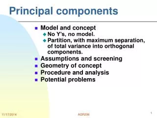
Principal components • Model and concept • No Y’s, no model. • Partition, with maximum separation, of total variance into orthogonal components. • Assumptions and screening • Geometry of concept • Procedure and analysis • Potential problems AGR206
Assumptions for PCA (1) • Normality. • Not required, but enhances results. • Multivariate normality can be tested by squared Mahalanobis distance. • D2~c2 (p) df=number of variables. • Extremely sensitive; use low a. • Linearity. • Assumed. • Can be inspected by scatterplots. • If violated, use transformation. AGR206
Assumptions of PCA (2) • Minimum number of cases. • Must be very large for fuzzy variables, and to yield general results. • T&F say 300; agricultural and biological papers published with 30 or more. • Outliers. • Very important to fix! • Outliers violate MV normality. • Identify by jackknifed squared Mahalanobis distance. • Transform or delete; fully document. AGR206
Analysis-SAS • proc princomp data=spartina out=spartpc;var h2s sal eh7 ph acid p k ca mg na mn zn cu nh4;run; • Output: • simple statistics by variable • Correlation matrix • Eigenvalues • Eigenvectors • Output file content: • same as original + all PC scores. AGR206
Eigenvalues • Eigenvalues are the variances of each PC. • They add up to total variance. • When based on correlation matrix (i.e. standardized variables) their sum equals the number of variables. • Their values can be used to identify the degree of collinearity and where is comes from. • Condition index or number (CN). • Square root of the largest l divided by l for the PC being considered. • CN>30 => problem for MLR (not PCA). AGR206
Spartina example Eigenvalues Eigenvalues of the Correlation Matrix Eigenvalue Difference Proportion Cumulative PRIN1 4.92391 1.22868 0.351708 0.35171 PRIN2 3.69523 2.08810 0.263945 0.61565 PRIN3 1.60713 0.27222 0.114795 0.73045 PRIN4 1.33490 0.64330 0.095350 0.82580 PRIN5 0.69160 0.19103 0.049400 0.87520 PRIN6 0.50057 0.11513 0.035755 0.91095 PRIN7 0.38544 0.00467 0.027531 0.93848 PRIN8 0.38077 0.21480 0.027198 0.96568 PRIN9 0.16597 0.02298 0.011855 0.97754 PRIN10 0.14299 0.05613 0.010214 0.98775 PRIN11 0.08687 0.04158 0.006205 0.99395 PRIN12 0.04529 0.01544 0.003235 0.99719 PRIN13 0.02985 0.02036 0.002132 0.99932 PRIN14 0.00949 . 0.000678 1.00000 AGR206
Eigenvectors • Coefficients that give the scores for each PC. • [PC] = Z V • Where: • [PC] is the matrix of PC scores; • Z is the matrix of standardized variables; • V is the matrix of eigenvectors. AGR206
Spartina [PC] = Z V Eigenvectors PRIN1PRIN2PRIN3PRIN4PRIN5PRIN6PRIN7 H2S -.163637 0.009086 0.231669 0.689722 0.014386 -.419348 0.300094 SAL -.107894 0.017324 0.605727 -.270389 0.508742 0.010076 0.383770 EH7 -.123813 0.225247 0.458251 0.301313 -.166758 0.596651 -.296867 PH -.408217 -.027467 -.282670 0.081726 0.091618 0.191256 0.056897 ACID 0.411680 -.000362 0.204919 -.165831 -.162713 -.024061 0.117085 P 0.273196 -.111277 -.160543 0.199965 0.747115 -.017903 -.336928 K -.033446 0.487887 -.022907 0.043000 -.061998 -.016587 -.067421 CA -.358562 -.180445 -.206595 -.054385 0.206152 0.427579 0.104949 MG 0.079033 0.498653 -.049515 -.036561 0.103793 0.034182 -.044195 NA -.017130 0.470439 0.050575 -.054358 0.239519 -.060440 -.181661 MN 0.277082 -.182164 0.019849 0.483078 0.038899 0.299511 0.124567 ZN 0.404195 0.088823 -.176373 0.150047 -.007768 0.034351 -.072907 CU -.010788 0.391707 -.376740 0.102023 0.063434 0.077993 0.562581 NH4 0.398754 -.025968 -.010607 -.104087 -.005857 0.381686 0.395252 PRIN8PRIN9PRIN10PRIN11PRIN12PRIN13PRIN14 H2S -.073755 0.168302 0.295840 0.222927 -.015407 0.006864 -.079812 SAL 0.100873 -.175066 -.227621 0.088425 -.156210 -.094878 0.089376 EH7 -.312742 -.226136 0.083754 -.023086 0.055421 -.033492 -.023123 PH -.029538 0.023918 0.146959 0.041662 -.331152 0.025938 0.750134 ACID -.152610 0.095416 0.101118 0.344782 0.455459 0.351392 0.477337 P -.398662 0.077828 -.017685 -.034542 0.064822 0.065467 0.014741 K -.115096 0.559085 -.555004 0.217893 -.030301 -.249524 0.072785 CA 0.185889 0.186412 0.073763 0.511310 0.346574 0.079545 -.307040 MG 0.170996 -.011293 0.111582 0.118799 -.397791 0.690127 -.192283 NA 0.449939 0.088170 0.439200 -.216233 0.363391 -.276211 0.143663 MN 0.531706 0.086117 -.361647 -.269913 0.077826 0.172893 0.140813 ZN 0.208525 -.439455 0.014406 0.568635 -.222750 -.396331 0.041311 CU -.277074 -.376706 -.129195 -.192872 0.305087 -.000372 -.043094 NH4 -.145025 0.420100 0.393717 -.130247 -.301510 -.230796 -.117317 AGR206
Loadings • Correlation between each variable and each PC. • For variable Zi (standardized)and PCj • r = lj0.5 vij • If based on covariances, use r = vij (sj/si) • Loadings represent the degree of association between the variable and the PC. • Loadings are used to create Gabriel’s biplot. AGR206
Gabriel’s Biplot AGR206
Potential problems • Depend on goal. • Detection of collinearity. • Reduction of dimensions. • Correlation or covariance matrix? • PC’s hard to interpret. • All l’s about the same size. • How many PC’s should be retained? • Scree plot. • Retain if l>average. • Retain as many necessary for 80%. AGR206
Scree plot AGR206

