Download
1 / 72
720 likes | 907 Vues
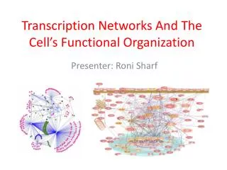
Discovery of transcription networks. Lecture3 Nov 2012 Regulatory Genomics Weizmann Institute Prof. Yitzhak Pilpel. Hierarchical clustering. CTCCTCCCCCCCTTC. TGGCCAATCA. ATGTACGGGTG. Promoter Motifs and expression profiles. CGGCCCCGCGGA. …HIS7. …ARO4. …ILV6. …THR4. …ARO1. …HOM2.

E N D
Discovery of transcription networks Lecture3 Nov 2012 Regulatory Genomics Weizmann Institute Prof. Yitzhak Pilpel
CTCCTCCCCCCCTTC TGGCCAATCA ATGTACGGGTG Promoter Motifs and expression profiles CGGCCCCGCGGA
…HIS7 …ARO4 …ILV6 …THR4 …ARO1 …HOM2 …PRO3 AlignACE Example 5’- TCTCTCTCCACGGCTAATTAGGTGATCATGAAAAAATGAAAAATTCATGAGAAAAGAGTCAGACATCGAAACATACAT 5’- ATGGCAGAATCACTTTAAAACGTGGCCCCACCCGCTGCACCCTGTGCATTTTGTACGTTACTGCGAAATGACTCAACG 5’- CACATCCAACGAATCACCTCACCGTTATCGTGACTCACTTTCTTTCGCATCGCCGAAGTGCCATAAAAAATATTTTTT 5’- TGCGAACAAAAGAGTCATTACAACGAGGAAATAGAAGAAAATGAAAAATTTTCGACAAAATGTATAGTCATTTCTATC 5’- ACAAAGGTACCTTCCTGGCCAATCTCACAGATTTAATATAGTAAATTGTCATGCATATGACTCATCCCGAACATGAAA 5’- ATTGATTGACTCATTTTCCTCTGACTACTACCAGTTCAAAATGTTAGAGAAAAATAGAAAAGCAGAAAAAATAAATAA 5’- GGCGCCACAGTCCGCGTTTGGTTATCCGGCTGACTCATTCTGACTCTTTTTTGGAAAGTGTGGCATGTGCTTCACACA 300-600 bp of upstream sequence per gene are searched in Saccharomyces cerevisiae. http://statgen.ncsu.edu/~dahlia/journalclub/S01/jmb1205.pdf
A cluster of gene may contain a common motif in their promoter 5’- TCTCTCTCCACGGCTAATTAGGTGATCATGAAAAAATGAAAAATTCATGAGAAAAGAGTCAGACATCGAAACATACAT …HIS7 …ARO4 5’- ATGGCAGAATCACTTTAAAACGTGGCCCCACCCGCTGCACCCTGTGCATTTTGTACGTTACTGCGAAATGACTCAACG …ILV6 5’- CACATCCAACGAATCACCTCACCGTTATCGTGACTCACTTTCTTTCGCATCGCCGAAGTGCCATAAAAAATATTTTTT 5’- TGCGAACAAAAGAGTCATTACAACGAGGAAATAGAAGAAAATGAAAAATTTTCGACAAAATGTATAGTCATTTCTATC …THR4 …ARO1 5’- ACAAAGGTACCTTCCTGGCCAATCTCACAGATTTAATATAGTAAATTGTCATGCATATGACTCATCCCGAACATGAAA …HOM2 5’- ATTGATTGACTCATTTTCCTCTGACTACTACCAGTTCAAAATGTTAGAGAAAAATAGAAAAGCAGAAAAAATAAATAA Find a needle in a haystack …PRO3 5’- GGCGCCACAGTCCGCGTTTGGTTATCCGGCTGACTCATTCTGACTCTTTTTTGGAAAGTGTGGCATGTGCTTCACACA AAAAGAGTCA AAATGACTCA AAGTGAGTCA AAAAGAGTCA GGATGAGTCA AAATGAGTCA GAATGAGTCA AAAAGAGTCA **********
Computational Identification of Cis-regulatory Elements Associated with Groups of Functionally Related Genes in Saccharomyces cerevisiae J.D. Hughes, P.W. Estep, S. Tavazoie, G.M. Church Journal of Molecular Biology (2000)
Motif Representation G1 A G A A G AG2 A A A T G AG3 G A A T G AG4 A G A A G AG5 A G A A G A Example GAL4 is one of the yeast genes required for growth on galactose. http://www.cifn.unam.mx/Computational_Genomics/old_research/BIOL2.html
Finding New Motif • By lab work • By comparison to known motifs in other species • By searching upstream regions of a set of potentially co-regulated genes
NCGTNNNNARTGAT CGATGAGMTK NCGTNNNNARTGAT&CGATGAGMTK The genes bound by the TF Abf1 can be clustered into several groups, some contain a motif (sporulation experiment)
Search Space • Size of search space: • L=600, W = 15, N = 10 : • Exact search methods are not feasible
AlignACE Example Input Data Set 5’- TCTCTCTCCACGGCTAATTAGGTGATCATGAAAAAATGAAAAATTCATGAGAAAAGAGTCAGACATCGAAACATACAT …HIS7 …ARO4 5’- ATGGCAGAATCACTTTAAAACGTGGCCCCACCCGCTGCACCCTGTGCATTTTGTACGTTACTGCGAAATGACTCAACG …ILV6 5’- CACATCCAACGAATCACCTCACCGTTATCGTGACTCACTTTCTTTCGCATCGCCGAAGTGCCATAAAAAATATTTTTT 5’- TGCGAACAAAAGAGTCATTACAACGAGGAAATAGAAGAAAATGAAAAATTTTCGACAAAATGTATAGTCATTTCTATC …THR4 …ARO1 5’- ACAAAGGTACCTTCCTGGCCAATCTCACAGATTTAATATAGTAAATTGTCATGCATATGACTCATCCCGAACATGAAA 5’- ATTGATTGACTCATTTTCCTCTGACTACTACCAGTTCAAAATGTTAGAGAAAAATAGAAAAGCAGAAAAAATAAATAA …HOM2 5’- GGCGCCACAGTCCGCGTTTGGTTATCCGGCTGACTCATTCTGACTCTTTTTTGGAAAGTGTGGCATGTGCTTCACACA …PRO3 300-600 bp of upstream sequence per gene are searched in Saccharomyces cerevisiae. Based on slides from G. Church Computational Biology course at Harvard
K-means • Start with random positions of centroids. • Assign data points to centroids. • Move centroids to center of assigned points. • Iterate till minimal cost. Iteration = 3
AlignACE Example Initial Seeding 5’- TCTCTCTCCACGGCTAATTAGGTGATCATGAAAAAATGAAAAATTCATGAGAAAAGAGTCAGACATCGAAACATACAT 5’- TCTCTCTCCACGGCTAATTAGGTGATCATGAAAAAATGAAAAATTCATGAGAAAAGAGTCAGACATCGAAACATACAT …HIS7 …ARO4 5’- ATGGCAGAATCACTTTAAAACGTGGCCCCACCCGCTGCACCCTGTGCATTTTGTACGTTACTGCGAAATGACTCAACG 5’- ATGGCAGAATCACTTTAAAACGTGGCCCCACCCGCTGCACCCTGTGCATTTTGTACGTTACTGCGAAATGACTCAACG …ILV6 5’- CACATCCAACGAATCACCTCACCGTTATCGTGACTCACTTTCTTTCGCATCGCCGAAGTGCCATAAAAAATATTTTTT 5’- CACATCCAACGAATCACCTCACCGTTATCGTGACTCACTTTCTTTCGCATCGCCGAAGTGCCATAAAAAATATTTTTT 5’- TGCGAACAAAAGAGTCATTACAACGAGGAAATAGAAGAAAATGAAAAATTTTCGACAAAATGTATAGTCATTTCTATC 5’- TGCGAACAAAAGAGTCATTACAACGAGGAAATAGAAGAAAATGAAAAATTTTCGACAAAATGTATAGTCATTTCTATC …THR4 …ARO1 5’- ACAAAGGTACCTTCCTGGCCAATCTCACAGATTTAATATAGTAAATTGTCATGCATATGACTCATCCCGAACATGAAA …HOM2 5’- ATTGATTGACTCATTTTCCTCTGACTACTACCAGTTCAAAATGTTAGAGAAAAATAGAAAAGCAGAAAAAATAAATAA 5’- GGCGCCACAGTCCGCGTTTGGTTATCCGGCTGACTCATTCTGACTCTTTTTTGGAAAGTGTGGCATGTGCTTCACACA …PRO3 TGAAAAATTC TGAAAAATTC GACATCGAAA GACATCGAAA GCACTTCGGC GCACTTCGGC GAGTCATTAC GAGTCATTAC GTAAATTGTC GTAAATTGTC CCACAGTCCG CCACAGTCCG TGTGAAGCAC TGTGAAGCAC MAP score = -10.0 Based on slides from G. Church Computational Biology course at Harvard
AlignACE Example Sampling Add? 5’- TCTCTCTCCACGGCTAATTAGGTGATCATGAAAAAATGAAAAATTCATGAGAAAAGAGTCAGACATCGAAACATACAT …HIS7 …ARO4 5’- ATGGCAGAATCACTTTAAAACGTGGCCCCACCCGCTGCACCCTGTGCATTTTGTACGTTACTGCGAAATGACTCAACG …ILV6 5’- CACATCCAACGAATCACCTCACCGTTATCGTGACTCACTTTCTTTCGCATCGCCGAAGTGCCATAAAAAATATTTTTT 5’- TGCGAACAAAAGAGTCATTACAACGAGGAAATAGAAGAAAATGAAAAATTTTCGACAAAATGTATAGTCATTTCTATC …THR4 …ARO1 5’- ACAAAGGTACCTTCCTGGCCAATCTCACAGATTTAATATAGTAAATTGTCATGCATATGACTCATCCCGAACATGAAA …HOM2 5’- ATTGATTGACTCATTTTCCTCTGACTACTACCAGTTCAAAATGTTAGAGAAAAATAGAAAAGCAGAAAAAATAAATAA 5’- GGCGCCACAGTCCGCGTTTGGTTATCCGGCTGACTCATTCTGACTCTTTTTTGGAAAGTGTGGCATGTGCTTCACACA …PRO3 TCTCTCTCCA TGAAAAATTC How much better is the alignment with this site as opposed to without? TGAAAAATTC GACATCGAAA GACATCGAAA GCACTTCGGC GCACTTCGGC GAGTCATTAC GAGTCATTAC GTAAATTGTC GTAAATTGTC CCACAGTCCG CCACAGTCCG TGTGAAGCAC TGTGAAGCAC Based on slides from G. Church Computational Biology course at Harvard
AlignACE Example Sampling Add? Remove. 5’- TCTCTCTCCACGGCTAATTAGGTGATCATGAAAAAATGAAAAATTCATGAGAAAAGAGTCAGACATCGAAACATACAT …HIS7 …ARO4 5’- ATGGCAGAATCACTTTAAAACGTGGCCCCACCCGCTGCACCCTGTGCATTTTGTACGTTACTGCGAAATGACTCAACG …ILV6 5’- CACATCCAACGAATCACCTCACCGTTATCGTGACTCACTTTCTTTCGCATCGCCGAAGTGCCATAAAAAATATTTTTT 5’- TGCGAACAAAAGAGTCATTACAACGAGGAAATAGAAGAAAATGAAAAATTTTCGACAAAATGTATAGTCATTTCTATC …THR4 …ARO1 5’- ACAAAGGTACCTTCCTGGCCAATCTCACAGATTTAATATAGTAAATTGTCATGCATATGACTCATCCCGAACATGAAA …HOM2 5’- ATTGATTGACTCATTTTCCTCTGACTACTACCAGTTCAAAATGTTAGAGAAAAATAGAAAAGCAGAAAAAATAAATAA …PRO3 5’- GGCGCCACAGTCCGCGTTTGGTTATCCGGCTGACTCATTCTGACTCTTTTTTGGAAAGTGTGGCATGTGCTTCACACA TGAAAAAATG TGAAAAATTC How much better is the alignment with this site as opposed to without? TGAAAAATTC GACATCGAAA GACATCGAAA GCACTTCGGC GCACTTCGGC GAGTCATTAC GAGTCATTAC GTAAATTGTC GTAAATTGTC CCACAGTCCG CCACAGTCCG TGTGAAGCAC TGTGAAGCAC Based on slides from G. Church Computational Biology course at Harvard
AlignACE Example Column Sampling 5’- TCTCTCTCCACGGCTAATTAGGTGATCATGAAAAAATGAAAAATTCATGAGAAAAGAGTCAGACATCGAAACATACAT …HIS7 …ARO4 5’- ATGGCAGAATCACTTTAAAACGTGGCCCCACCCGCTGCACCCTGTGCATTTTGTACGTTACTGCGAAATGACTCAACG …ILV6 5’- CACATCCAACGAATCACCTCACCGTTATCGTGACTCACTTTCTTTCGCATCGCCGAAGTGCCATAAAAAATATTTTTT 5’- TGCGAACAAAAGAGTCATTACAACGAGGAAATAGAAGAAAATGAAAAATTTTCGACAAAATGTATAGTCATTTCTATC …THR4 …ARO1 5’- ACAAAGGTACCTTCCTGGCCAATCTCACAGATTTAATATAGTAAATTGTCATGCATATGACTCATCCCGAACATGAAA …HOM2 5’- ATTGATTGACTCATTTTCCTCTGACTACTACCAGTTCAAAATGTTAGAGAAAAATAGAAAAGCAGAAAAAATAAATAA …PRO3 5’- GGCGCCACAGTCCGCGTTTGGTTATCCGGCTGACTCATTCTGACTCTTTTTTGGAAAGTGTGGCATGTGCTTCACACA How much better is the alignment with this new column structure? GACATCGAAA GACATCGAAAC GCACTTCGGC GCACTTCGGCG GAGTCATTAC GAGTCATTACA GTAAATTGTC GTAAATTGTCA CCACAGTCCG CCACAGTCCGC TGTGAAGCAC TGTGAAGCACA Based on slides from G. Church Computational Biology course at Harvard
AlignACE Example The Best Motif 5’- TCTCTCTCCACGGCTAATTAGGTGATCATGAAAAAATGAAAAATTCATGAGAAAAGAGTCAGACATCGAAACATACAT …HIS7 …ARO4 5’- ATGGCAGAATCACTTTAAAACGTGGCCCCACCCGCTGCACCCTGTGCATTTTGTACGTTACTGCGAAATGACTCAACG …ILV6 5’- CACATCCAACGAATCACCTCACCGTTATCGTGACTCACTTTCTTTCGCATCGCCGAAGTGCCATAAAAAATATTTTTT 5’- TGCGAACAAAAGAGTCATTACAACGAGGAAATAGAAGAAAATGAAAAATTTTCGACAAAATGTATAGTCATTTCTATC …THR4 …ARO1 5’- ACAAAGGTACCTTCCTGGCCAATCTCACAGATTTAATATAGTAAATTGTCATGCATATGACTCATCCCGAACATGAAA …HOM2 5’- ATTGATTGACTCATTTTCCTCTGACTACTACCAGTTCAAAATGTTAGAGAAAAATAGAAAAGCAGAAAAAATAAATAA …PRO3 5’- GGCGCCACAGTCCGCGTTTGGTTATCCGGCTGACTCATTCTGACTCTTTTTTGGAAAGTGTGGCATGTGCTTCACACA AAAAGAGTCA AAATGACTCA AAGTGAGTCA AAAAGAGTCA GGATGAGTCA AAATGAGTCA GAATGAGTCA AAAAGAGTCA MAP score = 20.37 Based on slides from G. Church Computational Biology course at Harvard
The MAP Score MAP • MAP – Maximal a priori log likelihood score • This is what the algorithm tries to optimize. • Measures the degree of over representation • of the motif in the input sequence relative to expectation in a random sequence.
The MAP Score B,G = standard Beta & Gamma functions N = number of aligned sites; T = number of total possible sites Fjb= number of occurrences of base b at position j (F = sum) Gb = background genomic frequency for base b bb = n x Gb for n pseudocounts (b = sum) W = width of motif; C = number of columns in motif (W>=C) Based on slides from G. Church Computational Biology course at Harvard
The MAP Score N = number of aligned sites exp = expected number of sites in the input sequence, comparing to a random model AGGGTAA P = 1 site every 16,000 bases For 64,000 bases sequence - exp = 4
Some examples Very intuitive: any things that’s long, that occurs many times and that is different from background will score highly
The MAP Score Properties • Motif should be “strong” • Input sequence can’t be too long AGGGTAA P = 1 site every 16,000 bases Genome length ~12Mb : Motif needs more than 1500 sites to get a positive MAP score: Problem: most transcription factor binding sites will only occur in dozens to hundreds of genes
Solution: Cluster genes before searching for motifs Time-point 1 Time-point 3 Time-point 2
ORFs with best sites (S2) Motif ORFs Group (S1) Group Specificity Score: All Genome (N) How well a motif targets the genes used to find it comparing to all genome ? What is the probability to have such large intersection? X N = Total # of ORFs in the genome (6226) S1 = # ORFs used to align the motif S2 = # targets in the genome (~ 100 ORFs with best ScanACE scores) X = # size of intersection of S1 and S2 Based on slides from G. Church Computational Biology course at Harvard
ORFs with best sites (S2) Motif ORFs Group (S1) Group Specificity Score: All Genome (N) How well a motif targets the genes used to find it comparing to all genome ? What is the probability to have such large intersection? X N = Total # of ORFs in the genome (6226) S1 = # ORFs used to align the motif S2 = # targets in the genome (~ 100 ORFs with best ScanACE scores) X = # size of intersection of S1 and S2 Based on slides from G. Church Computational Biology course at Harvard
Positional Bias Score: #ORFS10 6 1 50 bp Start -600 bp • Measures the degree of preference of positioning in a particular range upstream to translational start. Based on slides from G. Church Computational Biology course at Harvard
Positional Bias Score: #ORFS10 1 50 bp Start -600 bp • Find best 200 sites in the genome • Restrict sites to segment of length [s = 600 bp] from translation start • t = # sites in the segment • Choose window size [w = 50 bp] • m = # sites in the most enriched window • What is the probability to have m or more • sites in a window of size w? Based on slides from G. Church Computational Biology course at Harvard
Positional Bias Score: #ORFS10 1 50 bp Start -600 bp • Find best 200 sites in the genome • Restrict sites to segment of length [s = 600 bp] from translation start • t = # sites in the segment • Choose window size [w = 50 bp] • m = # sites in the most enriched window • What is the probability to have m or more • sites in a window of size w? Based on slides from G. Church Computational Biology course at Harvard
Lecture Topics • Introduction to DNA regulatory motifs • AlignACE - A motif finding algorithm • Assessment of motifs • AlignACE results on yeast genome • Summary & Conclusions
Comparisons of motifs • The CompareACE program finds best alignment between two motifs and calculates the correlation between the two position-specific scoring matrices • Similar motifs: CompareACE score > 0.7 Based on slides from G. Church Computational Biology course at Harvard
Pairwise CompareACE scores ABCD A 1.0 0.9 0.1 0.0 B 1.0 0.2 0.1 C 1.0 0.8 D 1.0 CompareACE Hierarchical Clustering cluster 1: A, B cluster 2:C, D Clustering motifs by similarity motif A motif B motif C motif D
Negative Controls • 250 AlignACE runs on randomly created groups of ORFs, of size 20, 40, 60, 80,and 100 ORFs. MAP MAP random real Based on slides from G. Church Computational Biology course at Harvard
Negative Controls MAP cut off of 10, Group Specificity cutoff of : False Positives = 10-20%
Positive Controls • 29 listed TFs with five or more known binding sites were chosen. • AlignACE was run on the upstream regions of the corresponding regulated genes. • An appropriate motif was found in 21/29 cases. • False negative rate = ~ 10-30 % Based on slides from G. Church Computational Biology course at Harvard
The data Organism: Saccharomyces cerevisiae Microarray experiment : Affymetrix microarrays of 6,220 mRNA Data: gathered by Cho et al. 15 time points, spanned about 4 hours across two cell cycles Genomesequence
Variance normalization and clustering of expression time series • 3,000 most variable ORFs were chosen (based on the normalized dispersion in expression level of each gene across the time points (s.d./mean). • The 15 time points were used to construct a 3,000 by 15 data matrix. • The variance of each gene was normalized across the 15 conditions: Subtracting the mean across the time points from the expression level of each gene and dividing by the standard deviation across the time point.
Before and after mean - variance normalization Before normalization After normalization
Representation of expression data Normalized ExpressionData from microarrays Time-point 1 Euclidean distance Gene 1 Gene 2
K-means • Start with random positions of centroids. = position of data point Xi = position of data centroid C Iteration = 0
Choosing K Sum Squared errors Since we don’t know the number of clusters in advance we need a way to estimate it. In order to choose the number of clusters K, the Sum of Squares of Errors is calculated for different K values. A clear break point indicates the “natural” number of clusters in the data. K
Significantly enrichment of functional category within clusters • Each gene was mapped into one of 199functional categories ( according to MIPS database ). • For each cluster, P-values was calculated for observing the frequencies of genes from particular functional categories. • There was significant grouping of genes within the same cluster.
The hyper-geometric score P values were calculated for finding at least (k) ORFs from a particular functional category within a cluster of size (n). where (f) is the total number of genes within a functional category and (g) is the total number of genes within the genome (6,220). P- values greater than 3×10- 4 are not reported, as their total expectation within the cluster would be higher than 0.05 As we tested 199 MIPS (ref.15).