Wireless Sensor Networks COE 499 Localization
Wireless Sensor Networks COE 499 Localization. Tarek Sheltami KFUPM CCSE COE www.ccse.kfupm.edu.sa/~tarek. Outline. Overview Key Issues Localization Approaches Coarse-grained node localization using minimal information. Overview.

Wireless Sensor Networks COE 499 Localization
E N D
Presentation Transcript
Wireless Sensor Networks COE 499Localization Tarek Sheltami KFUPM CCSE COE www.ccse.kfupm.edu.sa/~tarek
Outline • Overview • Key Issues • Localization Approaches • Coarse-grained node localization using minimal information
Overview • Each individual sensor observation can be characterized essentially as a tuple of the form <S, T, M>, where S is the spatial location of the measurement, T the time of the measurement, and M the measurement itself. The location needed for the following reasons: • To provide location stamps • To locate and track point objects • To monitor the spatial evolution of a diffuse phenomenon • To determine the quality of coverage. • To achieve load balancing • To form clusters • To facilitate routing • To perform efficient spatial querying • However, localization is only important in random deployment
Key Issues • What to localize? • The refers to identifying nodes have a priori known locations (called reference nodes) and which nodes do not (called unknown nodes) • The number and fraction of reference nodes in a network of n nodes may vary all the way from 0 to n−1 and could be static or mobile. The same applies to the unknown nodes • The unknown nodes can be cooperative or non-cooperative nodes • In case of non-cooperative scheme, nodes cannot participate in the localization algorithm
Key Issues.. • When to localize? • location information is needed for all unknown nodes at the very beginning of network operation • In static environments, network localization may thus be a one-shot process. • In other cases, it may be necessary to provide localization on-the-fly, or refresh the localization process as objects and network nodes move around, or improve the localization by incorporating additional information over time • The time scales involved may vary considerably from being of the order of minutes to days, even months
Key Issues.. • How well to localize? • The technique must provide the desired type and accuracy of localization, taking into account the available resources • How to localize? • The signals used can vary from narrowband radio signal strength readings or packet-loss statistics, UWB RF signals, acoustic/ultrasound signals, infrared • The signals may be emitted and measured by reference node, unknown nodes, or both • The basic localization algorithm may be based on a number of techniques, such as proximity, calculation of centroids, constraints, ranging, angulation, pattern recognition, multi-dimensional scaling, and potential methods
Cone-Based Topology Control Protocol • The authors claim that the protocol provides a minimal direction-based distributed rule to ensure that the whole network topology is connected, while keeping the power usage of each node as small as possible. • Protocol Description • Each node keeps increasing its transmit power until it has at least one neighboring node in every cone or it reaches its maximum transmission power limit • It is assumed here that the communication range increases monotonically with transmit power • CBTC showed that suffices to ensure that the network is connected • A tighter result has shown that can further reduced to
Localization approaches • Coarse-grained localization using minimal information: • Use a small set of discrete measurements, such as the information used to compute location • Minimal information could include binary proximity, near–far information • Fine-grained localization using detailed information: • Based on measurements, such as RF power, signal waveform, time stamps, etc. that are either real-valued or discrete with a large number of quantization levels • These include techniques based on radio signal strengths, timing information, and angulation • While minimal information techniques are simpler to implement, and likely involve lower resource consumption and equipment costs, they provide lower accuracy than the detailed information techniques
Coarse-grained node localization using minimal information • Binary proximity • A simple decision of whether two nodes are within reception range of each other • A set of references nodes are placed in the environment in some non-overlapping manner • Either the reference nodes periodically emit beacons, or the unknown node transmits a beacon when it needs to be localized • If reference nodes emit beacons, these include their location IDs, then unknown node must determine which node it is closest to, and this provides a coarse-grained localization • Alternatively, if the unknown node emits a beacon, the reference node that hears the beacon uses its own location to determine the location of the unknown node
Coarse-grained node localization using minimal information.. • Binary proximity.. • Examples: • Active Badge Location System • Radio Frequency Identification (RFID)
Coarse-grained node localization using minimal information.. • Centroid calculation • When the density of reference nodes is sufficiently high that there are several reference nodes within the range of the unknown node • In two dimensional scenario, let there be n reference nodes detected within the proximity of the unknown node, with the location of the ith such reference denoted by (xi, yi) • Let the location of the unknown node (xu, yu) • It is shown through simulations that, as the overlap ratio R/d is increased from 1 to 4, the average RMS error in localization is reduced from 0.5d to 0.25d
Coarse-grained node localization using minimal information.. • Geometric constraints • The region of radio coverage may be upper-bounded by a circle of radius Rmax • When both lower Rmin and upper bounds Rmax can be determined, based on the received signal strength, the shape for a single node’s coverage is an annulus • when an angular sector (θmin, θmax) and a maximum range Rmax can be determined, the shape for a single node’s coverage would be a cone with given angle and radius. • A computational simplification that can be used to determine this bounded region is to use rectangular bounding boxes as location estimates. Thus the unknown node determines bounds xmin, ymin, xmax, ymax on its position
Coarse-grained node localization using minimal information..
Coarse-grained node localization using minimal information.. • Approximate point triangle (APIT) • Similar to geometric constraints but the constraint region are defined as triangles between different sets of three reference nodes
Coarse-grained node localization using minimal information.. The approximate point-in-triange (APIT) technique
Coarse-grained node localization using minimal information.. Identifyingcodes Illustration of the ID-CODE technique showing uniquely identifiable regions