Routing Protocols

1. Routing Protocols RIP, OSPF, BGP

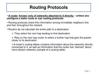
2. A Routing Protocol’s Job Is to Find a “Best” Path between Any Pair of Nodes • Routers in a network exchange their routing information using a routing protocol. • A routing table is set up in every router. • The routing table consists of many (destination host/network, next hop) entries. • When a packet arrives at a router, the router can look up the routing table to determine the next hop to forward the packet.

4. Routing Protocol Requirements • Minimize routing table space • Router’s memory is expensive. • The size of the Internet is huge! • Minimize control messages • Avoid wasting too much network bandwidth • Robustness • Avoid black holes • Avoid loops • Avoid oscillations • Using optimal paths • “Best” may mean (1) minimum number of hops, (2) least delay, (3) largest bandwidth, (4) least cost, or (5) others.

5. Choices • Centralized v.s. distributed • Source-based v.s. hop-by-hop • The header of a packet can carry (1) the addresses of every routers on the path from the source to the destination, or (2) just the address of the destination • QoS and resources can be reserved on the path • Two options: strict v.s. loose source routing • Has larger header overhead and may suffer the black holes problem

6. Choices (cont’d) • Stochastic v.s. deterministic • In stochastic method, packets can arrive at the destination out-of-order and/or with varying delay • Single v.s. multiple path • Internet uses the single path method for saving routers’ memory • State-dependent v.s. state-independent • In state-dependent routing, the choice of a route depends on the current network state (e.g., the loads, delays of links) • Good for load balancing and robustness but may have the loop, black hole, oscillation problems • State-independent routing (e.g., shortest-path routing) does not take the network state into account.

7. The Internet Uses a Two-Level Routing Approach • For management reasons, the Internet is divided into many autonomous systems (AS) connected together. • Routers in an AS use the same routing protocol. • Routes in an AS are managed by a single organization. • Routers in different ASes may use different routing protocols. • Interior Routing Protocols (e.g., RIP, OSPF) • Use within an AS • Exterior Routing protocols (e.g., BGP) • Exchange AS’s routing information between all ASes

9. Interior Routing Protocols

10. Distance Vector Routing Algorithm • Each router is configure with its own ID. • Each router is also configured with a number to use as the cost of each link. • Each router starts with a distance vector consisting of the value 0 for itself and the value infinity for every other destination. • Each router transmits its distance vector to each of its neighbor whenever the information changes. • Each router saves the most recently received distance vector from each of its neighbors. RIP uses DV.

11. Distance Vector Routing Algorithm (cont’d) • Each router calculates its own distance vector, based on minimizing the cost to each destination, by examining the the cost to that destination reported by each neighbor in turn and then adding the configured cost of the link to that neighbor. • The following events cause recalculation of the distance vector. • Receipt from a neighbor of a distance vector containing different information than before. • Discovery that a link to a neighbor has gone down. In that case, the distance vector from that neighbor is discarded before the distance vector is recalculated. The above uses Triggered Update, to prevent generating tom many control messages, we can use non-Triggered Update.

12. An Example of DVR Operation

13. The “Count-to-Infinity” Problem of DVR • Initially, on node B, the cost to C is 1. On node A, the cost to C is 2. • When the link between B and C breaks, B thinks that its shortest path to C is through A and now the cost becomes 1 + 2 = 3. • Because B’s distance vector has changed, B sends the newest information to node A. • Now A thinks that the cost to C becomes 1+3 = 4. • This process repeats until the infinity is reached and then both nodes realize there is no route to C.

14. The Effects of the “Count-to-Infinity” Problem • Slow down route convergence. • When the network topology has changed, the routing protocol cannot immediately change the routing table to reflect the new topology. • Loops now are formed. Packets are sent in a circle wasting network bandwidth • What value should be used for “Infinity”? • Too small, good packets may be discarded if they need to traverse many hops. • Too large, the “count-to-infinity” problem may last too long and in the mean times, many packets will be trapped in the routing loops.

15. Many Solutions to the “Count-to-Infinity” Problems • Hold-down • If the path you are using to D does down, you wait for some time before switching to another path. At the same time, you advertise your cost to D as infinity. • Slow convergence. • Reporting the entire path instead of just the next hop • By checking the entire routing path to the destination, we can detect routing loops. • Too expensive.

16. Many Solutions to the “Count-to-Infinity” Problems (Cont’d) • Split horizon • A router never advertises the cost of a destination to its neighbor N, if N is the next hop to that destination. • This solves many cases. However, it cannot solve some cases such as the following case.

17. Many Solutions to the “Count-to-Infinity” Problems (Cont’d) • Triggered update • In non-Triggered update, new distance vector information is exchanged once every 30 seconds. This takes too much time before the the “count-to-infinity” problem to be detected. • Triggered update speeds up the detection of the “count-to-infinity” problem at the cost of more control messages and more oscillations.

18. Many Solutions to the “Count-to-Infinity” Problems (Cont’d) • Source tracing • Augment a distance vector so that it carries not only the cost to a destination, but also the router immediately preceding the destination. • The purpose is to be able to construct the entire routing path to a destination without carrying the it. • Once we have the entire routing path, we can detect routing loops.

19. Link State Routing Algorithm • Each router is responsible for meeting its neighbors and learning their names. • Each router constructs a packet known as a link state packet, or LSP, which contains a list of names of the cost to each of its neighbors. • The LSP is somehow transmitted to all the other routers, and each router stores the most recently received generated LSP from each other router. • Each router, armed with a complete map of the topology, computes routes to each destination. OSPF uses LSR.

20. Link State Routing Algorithm (Cont’d) • Meeting neighbors • Send special packets over a link to identify themselves • Constructing an LSP • A router R generates an LSP periodically as well as when R discovers that • It has a new neighbor. • The cost of the link to an existing neighbor has changed. • A link to a neighbor has gone down.

21. Link State Routing Algorithm (Cont’d) • Disseminating the LSP to all routers • The most critical and difficult part of LSR. • If it is not done right, • Different routers in a network may have different views of the network, causing back holes, routing loops, oscillations to happen. • The LSP distribution may become cancerous, causing all network resources to be spent on processing LSPs. • Disseminating LSPs to other routers cannot rely on the routing protocols that is being used. • This causes the chicken-or-the-egg problem. • We need to use a more primitive method. • Flooding.

22. Flooding Guarantees That Every Router Receives a LSP • When a router receives a packet from a link, for each other link, it makes a copy of the packet and send it out. • The number of copies of the packet in the network grows exponentially like cancer.

23. An Improved Flooding Method • Use TTL (hop count) to prevent a packet’s endless spawning. • If a router R keeps the most recently generated LSP from each router S, R can recognize when it is receiving a duplicate of S’s most recently generated LSP, and refrain from flooding the packet more than once. • Sounds good. Now the problem becomes how does a router know which LSP is the most recently generated LSP (not the most recently received LSP – not always the most recently generated LSP due to network queueing delay, or taking different path) from a router S?

24. Timestamp or Sequence Number Can Help Routers To Determine Which LSP Is More Recently Generated. • A router can put a timestamp or a sequence number into its LSP so that other routers can which LSP is more recently generated. • What if, due to router bugs or signal errors, the timestamp or the sequence number jumps to 15 years later? • Also, the number of bits used to represent either timestamp or sequence number is limited (16 or 32). The timestamp or sequence number will wrap back.

25. The Method Used to Compare Two Sequence Numbers • Two sequence numbers a and b between [0 and n]: • a is considered to be less than b if |a –b| < n/2 and a < b or |a - b| > n/2 and a > b.

26. Age Limits the Effect of a Bad LSP • If we set an age in a LSP indicating the length of the period in which this LSP is considered as valid, a bad LSP (e.g., a timestamp that jumps 15 years into the future) will be purged away after some time (e.g., after 1 hour) • Also, a router R that wants all other routers to discard its current LSP, can send a LSP with the currently highest sequence number and 0 as its age value.

27. LSR Use Dijkstra’s Algorithm to Compute One-to-Many Shortest Paths

29. Comparison of LSR and DV • Nowadays, OSPF (using LSR) is more popular than RIP (using DV) • Convergence speed • LSR is better than DV • A router propagates a LSP before updating its routing table. • Functionality • LSR supports more functionality. (because it has the global network topology) • Robustness • LSR is better. (because it has the global network topology) • Computation cost • Roughly the same • Bandwidth consumed • Different results for different cases • Memory • The same. (k * n)

30. Exterior Routing Protocol

31. Border Gateway Protocol (BGP):A Path Distance Vector Routing Protocol • Those routers that are at the border of an AS and connect to other routers in another AS are called “border gateway”. • Border gateways of different ASes exchange their routing information. • BGP uses various policies to determine the routing path for different traffic. E.g., • If the packet comes from Pentagon, do not let it traverse an AS in Iraq • If the packet comes from Toronto and destines to Vancouver, do not let it traverse an AS in US • If the packet comes from HINET, do not let it use my ASes.

32. BGP Message Format AS_Path: A list of ASes that are traversed for this route. Next_Hop: The IP address of the border router that should be use as the next hop to the destination listed in NLRI. NLRI: consists of a list of network addresses

33. Example AS_Path: AS2 Next_Hop: R5 NLRI: 2.1, 2.2, 2.3, 2.4 AS_Path: AS2, AS1 Next_Hop: R5 NLRI: 1.1, 1.2, 1.3, 1.4 R9 AS_Path: AS1 Next_Hop: R1 NLRI: 1.1, 1.2, 1.3, 1.4