Download
1 / 1
10 likes | 147 Vues
Long term observations of climate altering gases for deriving emissions on a regional scale. Michela Maione 1 , Umberto Giostra 2 , Francesco Furlani 2 , Jgor Arduini 1 1 University of Urbino, Institute of Chemical Sciences , 2 University of Urbino, Institute of Physics ,

E N D
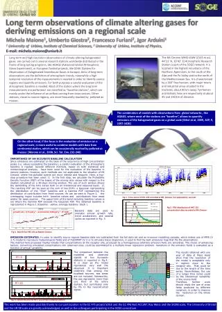
Long term observations of climate altering gases for deriving emissions on a regional scale Michela Maione1, Umberto Giostra2, Francesco Furlani2, Jgor Arduini1 1 University of Urbino, InstituteofChemicalSciences, 2 University of Urbino, InstituteofPhysics, E-mail: michela.maione@uniurb.it Long term and high resolution observations of climate altering halogenated gases are carried out in several research stations worldwide distributed in the frame of long lasting programs, like AGAGE (Advanced Global Atmospheric Gases Experiment), or European funded projects, like SOGE (System for Observation of Halogenated Greenhouse Gases in Europe).Aims of long term observations are the definition of atmospheric trends, meanwhile a high temporal resolution of the measurements is needed in order to identify source regions and quantify emissions. For both purposes a careful evaluation of the atmospheric baseline is needed. Most of the station where the long term measurements are performed are classified as “baseline stations”, which are mainly under the influence of an airflow coming from clean sectors. Other stations, closer to source regions, are more frequently reached by polluted air masses. The Mt Cimone WMO-GAW (2165 m asl, 44°11’ N, 10°42’ E) Atmospheric Research Station is part of the SOGE network. It is located in the highest mountains of the Northern Apennines, to the south of the Alps and the Po Valley and to the north of the Mediterranean Sea. It is characterized by a 360° free horizon, with major towns and industrial areas situated in the lowlands, about 40 km away; Tyrrhenian and Adriatic Seas are respectively at about 45 and 130 km of distance. The combination of models with observations from global networks , like AGAGE, where most of the stations are “baseline”, allows to quantify emissions of the halogenated gases on a global scale [Sthol et al, 2009, ACP, 9, 1597-1620] On the other hand, if the focus is the evaluation of emission on a regional scale, is more useful to combine models with data from continental station, which can be occasionally reached by polluted air masses [Maione et al., 2008, Sci. Tot. Env, 232-240] IMPORTANCE OF AN ACCURATE BASELINE CALCULATION Since emissions are estimated on the base of the occurrence of high concentration peaks (i.e. values exceeding the baseline), a careful evaluation of the atmospheric baseline is needed. Several different methods, based on both statistical and meteorological analysis, have been used for the evaluation of the baseline in remote stations. However, such methods are not applicable to the situation of Mt Cimone, where the polluted events are more intense and frequent. Here, a two-step procedure has been used: 1) In the first step, we calculate the Probability Density Function (PDF) of the biases of the mixing ratio values with respect to the median calculated on a 30-days moving window. The use of such window allows the detrending of the time series both on an interannual and seasonal basis. 2) The resulting PDF can be seen as the sum of two PDFs: a Gaussian representing the distribution of the “final” baseline and a Gamma PDF representing the distribution of contribution from fresh sources. As can be seen in Figure 2, the overlapping region includes both baseline values and contributions from weak and/or far away sources . The upper limit of the band including baseline values is set where the Gamma PDF exceeds the Gaussian PDF. The obtained baseline is represented in Figure 1 (baseline : yellow, average baseline: black ). Fig 1. Time series of HFC-125 recorded at Mt. Cimone. For explanation, see text Fig 2. PDF distribution of HFC-125 concentration data recorded at Mt.Cimone growth rate: 0.75 ppt y-1 -acceleration0.08 ppt y-2 - R2 0.98 Baseline data are used to evaluate annual growth rate, trend acceleration, and sesonal cycles as reported in Fig. 3 Fig 3. Best fit for HFC-125 at Monte Cimone EMISSION ESTIMATES. In order to identify source regions baseline data are subtracted from the full data set and an inversion modelling cascade, which makes use of MM5 (V 3.7) model to reproduce meteorological fields and of FLEXPART (V 3.1) to simulate tracer dispersion, is used to find the best emissions map that fits the observations. The method here proposed implies initially that concentrations at the receptor site, produced by a homogeneous arbitrary emission field, are simulated. The choice of enhancing factors, converting simulated concentrations into observed ones, could be assimilated to a multiple linear regression problem. Variations in the emission fields is evaluated as a function of annual variability. The comparison between the modelled and observed signals at two European stations is reported in Fig.4. It is clear as the model reproduces very well the observed. It is important underline that among the localised sources, sea areas are not included. Noteworthy, the sea represents more than one third of the entire domain, but contributes only by 3% to the reconstructed signal. The results obtained with one year of data at Mace Head show that the resolution of the model is acceptable only in regions close to the receptor site. That could be due to the length of the time series. Nevertheless, the use of a longer time series could be the interannual variability of the source field. Therefore, further work should imply the use of cross fields produced by different receptors, in order to improve the resolution on the whole domain. R2=.8 R2=.65 Fig. 4: Sensitivity test for HFC-125 at two European Station This work has been made possible thanks to our participation in the EC FP5 project SOGE and the EC FP6 NoE ACCENT. Ray Weiss and the SIO98 scale, The University of Bristol and the UB 98 scale are greatly acknowledged, as well as the colleagues participating in the SOGE consortium.