Download
1 / 37
380 likes | 426 Vues
Genetics and Genetic Prediction in Plant Breeding. Class Test #2, March, 1998. Eight Questions worth 100 points total Bonus Point worth 10 points Show all calculations 50 minutes. Question 1a.

E N D
Class Test #2, March, 1998 Eight Questions worth 100 points total Bonus Point worth 10 points Show all calculations 50 minutes
Question 1a Assuming an additive/dominance mode of inheritance for a polygenic trait, list expected values for P1, P2, and F1 in terms of m, [a] and [d]. [3 points] P1 = m + a P2 = m – a F1 = m + d
Question 1b From these expectations, what would be the expected values for F2, B1 and B2 based on m, [a] and [d]. [3 points] F2 = m + ½d B1 = m + ½a + ½d B2 = m – ½a + ½d
Question 1c From a properly designed field trial that included P1, P2 and F1 families, the following yield estimates were obtained. P1 = 1928 Kg; P2 = 1294 Kg; F1 = 1767 Kg From these family means, estimate the expected value of F2, B1, B2 and Fα, based on the additive/dominance model of inheritance [3 points].
Question 1c P1 = 1928 Kg; P2 = 1294 Kg; F1 = 1767 Kg a = [P1 – P2]/2 = [1928-1294]/2 = 317 m = [P1 – a] = 1928 – 317 = 1611 d = [F1 – m] = 1767 – 1611 = 156 F2 = m + ½d = 1611 + 78 = 1689 B1 = m+½a+½d = 1611+158.5+78 = 1397.5 B2 = m–½a+½d = 1611-158.5+78 = 1530.5
Question 2 A spring barley breeding program has major emphasis in developing cultivars which are short in stature and with yellow stripe resistance. It is known that the inheritance of short plants is controlled by a single completely recessive gene (tt) over tall plants (TT), and that yellow stripe rust resistance is controlled by a single completely dominant gene (YY), over a recessive susceptible gene (yy). The tall gene locus and yellow rust gene locus are located on different chromosomes. Given that a tall resistant plant (TTYY) is crossed to a short susceptible plant (ttyy), both parents being homozygous, what would be the expected proportion of genotypes and phenotypes in the F1 and F2 families [12 points].
Tall, Res. (TTYY) x Short, Susc. (ttyy) F1 TtYy Tall/Resistant
Tall, Res. (TTYY) x Short, Susc. (ttyy) 1 TTYY:2TTYy:1 TTyy:2 TtYY:4 TsYy:2Ttyy:1ttYY:2 ttYy:1 ttyy
Tall, Res. (TTYY) x Short, Susc. (ttyy) 9 T_Y_ : 3 T_yy : 3 ttY_ : 1 ttyy
Question 2 How many F3 plants would need to be assessed to ensure, with 99% certainty, that at least one plant would exist that was short and homozygous yellow rust resistant (i.e. ttYY) [8 points]. ttYY = 9/64 = 0.1406 # = Ln[1-0.99] = Ln(0.01) Ln[1-0.1406] Ln(0.8594) = 30.39, need 31 F3 plants
Question 3a Two genetically different homozygous lines of canola (Brassica napus L.) were crossed to produce F1 seed. Seed from the F1 family was self pollinated to produce F2 seed. A properly designed experiment was carried out involving both parents (P1 and P2, 10 plants each), the F1 (10 plants) and the F2 families (64 plants) was grown in the field and plant height of individual plants (inches) recorded. The following are family means, variances and number of plants observed for each family Family Mean Variance # Plants P1 52 1.97 10 P2 41 2.69 10 F1 49 3.14 10 F2 43 10.69 34 Complete a statistical test to determine whether an additive/dominance model of inheritance is appropriate to adequately explain the inheritance of plant height in canola [7 points].
Question 3a C-scaling test = 4F2– 2F1 – P1 – P2 C = 172-98-52-41 = 19 V(C) = 16V(F2)+4V(F1)+V(P1)+V(P2) V(C) = 171.04+12.56+1.97+2.69 = 188.26 se(C) = 188.26 = 13.72
Question 3a C = 172-98-52-41 = 19 se(C) = 188.26 = 13.72 t90df = 19/13.72 = 1.38 ns Therefore, additive/dominance model is adaquate
Question 3a P1 52 P2 41 m 46.5 F2 43 F1 49 ?
Question 3b If the additive/dominance model is inadequate, list three factors which could cause the lack of fit of the model [3 points]. • Abnormal chromosomal behavior: where the heterozygote does not contributes equal proportions of its various gametes to the gene pool. • Cytoplasmic inheritance: where the character is determined by non-nuclear genes. • Epistasis: where alleles at different loci are interacting.
Question 4a F1, F2, B1, and B2 families were evaluated for plant yield (kg/plot) from a cross between two homozygous spring wheat parents. The following variances from each family were found: σ2F1= 123.7; σ2F2= 496.2; σ2B1= 357.2; σ2B2= 324.7 Calculate the broad-sense (h2b) and narrow-sense (h2n) heritability for plant yield [10 points].
Question 4a σ2F1= 123.7; σ2F2= 496.2; σ2B1= 357.2; σ2B2= 324.7 h2b = Genetic variance Total variance E = V(F1) = 123.7 h2b = 496.2 – 123.7 496.2 h2b = 0.75
Question 4a σ2F1= 123.7; σ2F2= 496.2; σ2B1= 357.2; σ2B2= 324.7 E = V(F1) = 123.7 D = 4[V(B1)+V(B2)-V(F2)-E] 4[357.2+324.7-496.2-123.7] = 248 A = 2[V(F2)-¼D-E] = 2[496.2-62-123.7] = 621 h2n = ½A/V(F2) = 310.5/496.2 = 0.63
Question 4b Given the heritability estimates you have obtained, would you recommend selection for yield at the F3 in a wheat breeding program, and why? [2 points]. A narrow-sense heritability greater than 0.6 would indicate a high proportion of the total variance was additive in nature. Selection at F3 is often advesly related to dominant genetic variation (caused by heterozygosity), here D is small compared to A. Additive genetic variance is constant over selfing generations and so selection would result in a good response.
Question 5a Four types of diallel crossing designs have been described by Griffing. Briefly outline the features of each Method 1, 2, 3, and 4 [4 points]. 1. Complete diallel with selfs, Method 1. 2. Half diallel with selfs, Method 2. 3. Complete diallel, without selfs, Method 3. 4. Half diallel, without selfs, Method 4.
Question 5a Why would you choose Method 3 over Method 1? [1 point]. In instances where it was not possible to produce selfed progeny (i.e. in cases of strong self-incompatibility in apple and rapeseed). Why would you choose Method 2 over Method 1? [1 point]. In cases where there is no recipricol or maternal effects.
Question 5b A full diallel, including selfs is carried involving five chick-pea parents (assumed to be chosen as fixed parents), and all families resulting are evaluated at the F1 stage for seed yield. The following analysis of variance for general combining ability (GCA), specific combining ability (SCA) and reciprocal effects (Griffing analysis) is obtained:
Question 5b GCA is significant at the 99% level, while SCA and reciprical differences were not significant. This indicates that a high proportion of phenotypic variation between progeny is additive rather than dominant or error.
Question 5b If a random model is chosen then the GCA term is tested using the SCA mean square. In this case the GCA term is not formally significant, and the indication overall would be that there is no significant variation between progeny in the diallel.
Question 5b Plant height was also recorded on the same diallel families and an additive/dominance model found to be adequate to explain the genetic variation in plant height. Array variances Vi's and non-recurrent parent covariances (Wi's) were calculated and are shown along-side the general combining ability (GCA) of each of the five parents, below:
Question 5b Visual inspection of Vi and Wi values would indicate a linear relationship with slope approximatly equal to 1, which would indicate a additive/dominance model of inheritance. Parents with lowest Vi and Wi values (those with greatest frequency of dominant alleles) have negative GCA values indicating short stature in chick pea is dominant over tall stature.
Question 6a Two homozygous barley parents were crossed to produce an F1 family. One parent was tall with awns and the other was short and awnless. Tall plants are controlled by a single dominant gene and awned plants are also controlled by a single dominant gene. The F1 family was crossed to a plant which was short and awnless and the following number of phenotypes observed:
Question 6a % Recombination [259+221]/2400 = 0.20
16 TTAA:8TTAa:1 TTaa:8 TtAA:34 TtAa:8Ttaa:1ttAA:8 ttAa:16 ttaa 66 T_A_ : 9 T_aa : 9 ttA_ : 16 ttaa
Question 6a What is the difference between linkage and pleiotropy? [2 points]. Linkage is when alleles at two loci do not segregate independantly and hence there is linkage disequilibrium in segregating populations. The cause is that the two loci are located on the same chromosome. Pleiotropy is where two characters are controlled by alleles at a single locus.
Question 7a Two homozygous squash plants were hybridized and an F1 family produced. One parent was long and green fruit (LLGG) and the other was round and yellow fruit (llgg). 1600 F2 progeny were examined from selfing the F1's and the following number of phenotypes observed: Explain what may have caused this departuure from a 9:3:3:1 expected frequency of phenotypes [4 points].
Question 7a Explain what may have caused this departuure from a 9:3:3:1 expected frequency of phenotypes [4 points]. This departure from a 9:3:3:1 ratio could be caused by recessive epistasis, where ll is epistatic to G, so llG_ and llgg have the same phenotype.
Question 7a A appropriate test to use would be a chi-square test.
Bonus Question A 4x4 half diallel (with selfs) was carried out in cherry and the following fruit yield of each possible F1 family observed. Calculate narrow-sense heritability.
Bonus Question SS(x) = x2 – (x)2/n = 153.0 SP(x,y) = xy – (x y)/n = 130.5 b = 130.5/153.0 = 0.8529 = h2n
The End Thank you all Good Luck on Friday