Efficient Cost Estimation for Relational Algebra Queries: Strategies and File Structures
370 likes | 526 Vues
This document discusses cost estimation techniques for relational algebra queries, focusing on data retrieval strategies based on the type of query and file structure. It outlines the different query types including exact matches, range queries, and unordered prints, while reviewing file structures such as unsorted data files, sorted data files, and various indexing methods like B-trees and hash tables. Metrics important for understanding query costs are also examined, enabling users to choose the most efficient data retrieval method to minimize disk access and optimize performance.

Efficient Cost Estimation for Relational Algebra Queries: Strategies and File Structures
E N D
Presentation Transcript
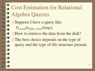
Cost Estimation for Relational Algebra Queries • Suppose I have a query like P(ename)[s(ID# = 1234)(Emp)] • How to retrieve the data from the disk? • The best choice depends on the type of query and the type of file structure present.
Simple Query Types • Exact matches on a unique attribute. • Exact matches on a non-unique attribute. • Range queries. • Print the entire file unordered. • Print the entire file, sorted on a particular attribute.
Possible File Structures • Access unsorted data file. • Access sorted data file. • Use an index/b-tree/b+-tree (“Secondary Index” or “Alternative 2/3”) • Use a hash table • Use a clustered B-Tree (“Primary Index” or “Alternative 1”) • Use clustered files.
Cost Estimation Introduction • To determine the best choice, we must have a way of determining the cost of each of the previous file structure access schemes with all of the possible query types. • This requires we understand how files are stored and retrieved from secondary storage.
File Systems Review: • A table will be stored as a file; the following metrics should be review: • r --the number of records in the file. • |r| -- the size of a record, usually bytes/record. • Block Size -- the number of bytes/block on the disk. A block is the number of bytes that can be read with one disk access. • bf -- the blocking factor of the file. It is the ëBlock Size/|r|û Note: ë û represents the floor function.
File Systems Review II: • b -- the number of blocks needed for the file. It is ér/ bfù. Note: éù represents the ceiling function. • For a b-tree, the number of levels in the tree is L. This is important because each level must be accessed once for a simple search (worst case). • Also in a b-tree the maximum number of levels is given by: • L <= log ém/2ù((N+1)/2) + 1 where m is the degree of the tree, and N is the number of key values.
Finding m: • |node| <=block size • (m-1)*|key| + (m)*|ChildPtr| + (m-1)*|RecPtr| <= block size
File Systems Review III: • bL is the number of nodes of a B-tree at the terminal level. This is important for determining the number of disk accesses for non-unique retrievals. • “d” is the number of distinct values of a particular attribute. • “s” is the selectivity of a particular attribute. It is r/d.
Cost Estimation -- Unsorted File • CUu = b (worst case) b/2 (average case). • CUn = b • CUr = b • CUpu = b • CUps = b log (b) + b
Cost Estimation -- Sorted File • CSu = log(b) • CSn = log(b) + és/bf ù - 1 • CSr = log(b) + b/2 • CSpu = b • CSps = b
Cost Estimation -- B-, B+-tree (Secondary) • CBu = L+1 • CBn = L+ (és/(m-1) ù - 1) + s • CBr = L+ bL/2 + r/2 • CBpu = L + bL + r • CBps = L + bL + r
Cost Estimation -- B-, B+-tree (Primary) • CBPu = L • CBPn = L+ (és/(m-1) ù - 1) • CBPr = L+ bL/2 • CBPpu = L + bL • CBPps = L + bL
Cost Estimation -- Hash Table • CHu = 1+1 = 2 • CHn = 1+s • CHr = NA • CHpu = #bins + r • CHps = NA
Cost Estimation -- Clustered Files • CCu = log(bR+bS) • CCn = log(bR+bS) + és/bf ù - 1 • CCr = log(bR+bS) + (bR+bS)/2 • CCpu = bR+bS • CCps = bR+bS • Clustered files are used to speed up joins, so these would be worse than a sorted file by design.
Example -- File Information • Emp(Fn, Minit, LN, SSN, Bdate, Addr, Sex, Salary, SuperSSN, Dno) • r = 10,000 records • bf = 5 records/block • b = 2,000 blocks • Hash Table on SSN • B+-Tree on Dno: • Ldno = 4, ddno = 125, sdno= 80, mdno = 50 • BLdno = 200
Example -- File Information II • B+-Tree on Salary: • Ldno = 4, ddno = 10,000, sdno= 1, mdno = 45 • BLdno = 250
Example -- The Queries • sssn = 1234(Emp) • sDno = 5(Emp) • sDno > 5(Emp) • sDno = 5 Ù Salary =30000 Ù Sex = ‘F’ (Emp)
Example -- Query #1 sssn = 1234(Emp) • How can we perform this query? • Access the EMP table unsorted: • CUu = b = 2,000 disk accesses • Use the Hash table on SSN: • CHu = 2 • Best choice: • Use the hash table.
Example -- Query #2 • sDno = 5(Emp) • How can we perform this query? • Access the EMP table unsorted: • CUn = b = 2,000 disk accesses • Use B+-Tree on Dno: • CBn = L+ (és/m ù - 1) + s = 4 + 1 + 80 = 85 • Best Choice: • Use the B+-Tree.
Example -- Query #3 sDno > 5(Emp) • How can we perform this query? • Access the EMP table unsorted: • CUr = b = 2,000 disk accesses • Use B+-Tree on Dno: • CBr = L+ bL/2 + r/2 = 4 + 100 + 5000 = 5104 • Best Choice: • Use the unsorted file.
Example -- Query #4 • sDno = 5 Ù Salary = 30000 Ù Sex = ‘F’ (Emp) • How can we perform this query? • Access the EMP table unsorted: • CUn = b = 2,000 disk accesses • Use B+-Tree on Dno = 85 disk accesses • Then apply remaining conjuncts to result in memory.
Example -- Query #4 (cont) • Use B+-Tree on Salary: • CBn = L+ (és/m ù - 1) + s = 4 + 0 + 1 = 5 • Use unsorted file access for Sex = ‘F’: • CUn = b = 2,000 • Which is best? • Use B+-Tree on salary, then apply the others to result in memory.
Join Cost Functions • Suppose I have R ê S. How do I estimate the cost of this? a=b • CJ1: Nested Loop Approach: • Access the blocks of R and for each record, access the blocks of S looking for matches. • CJ1 = bR + bR * bS + Write-to-disk-cost
Join Cost Functions II • CJ2: Use B-Tree (for example) on S.b: • Access each block of R, then search the B-Tree looking for matches. • CJ2 = bR + rR * (LS.b + SS.b)+ WTDC • Note: Using a B-Tree on R.a and accessing the blocks of S first could yield a different cost.
Join Cost Functions III • CJ3: If the two files are clustered: • CJ3 = bR + bS + WTDC
Write to Disk Cost • WTDC is the cost to write an intermediate result to disk. This would be the number of blocks in the resulting table. • WTDC = |RêS| / BFRêS • I need |RêS|, but this is hard to calculate directly. • The “Join Selectivity” is easier to estimate: • JS = |RêS| / |R ´ S|
Join Selectivity • JS = |RêS| / |R ´ S| • JS = |RêS| / |R| ´ |S| • |RêS| = JS ´ |R| ´ |S| • WTDC = |RêS| / BFRêS • WTDC = JS ´ |R| ´ |S| / BFRêS
Join Selectivity II • Note: if R.a is the key of R, then |RêS| <= |S| • WTDC <= |S| / BFRêS
Example Join-- File Information • Emp(Fn, Minit, LN, SSN, Bdate, Addr, Sex, Salary, SuperSSN, Dno) • r = 10,000 records • bf = 5 records/block • b = 2,000 blocks • B+-Tree on Dno: • Ldno = 4, ddno = 125, sdno= 80, mdno = 50 • BLdno = 200
Example Join-- File Information • Dept(D#, Dname, MGRSSN, MgrStartDate) • r = 125 records • bf = 10 records/block • b = 13 blocks • B+-Tree on D#: • Ldno = 2, ddno = 125, sdno= 1, mdno = 50 • BLdno = 3
The Sample Query: • I want to use Emp ê Dept. What are my options? Dno=D# • Nested Loop approach. • Use B-Tree on Emp.Dno. • Use B-Tree on Dept.D# • Cluster Employee and Department together.
Join Query -- Nested Loop Emp ê Dept. Dno=D# • CJ1 = bEmp * bDept = 2000 * 13 = 26,000
Join Query -- B-Tree on D# Emp ê Dept. Dno=D# • CJ2D# = bEmp + rEmp * (LDept.D# + SDept.D#) = 2000 + 10000 * (2 + 1) = 32,000
Join Query -- B-Tree on Dno Emp ê Dept. Dno=D# • CJ2D# = bDept + rDept * (LEmp.Dno + SEmp.Dno) = 13 + 125 * (4 + 80) = 10,513 • This is the better choice. • Note: I have ignored the WTDC here because it would be the same in all cases.
Join Query -- Clustered Files Emp ê Dept. Dno=D# • CJ3 = bR + bs = 2000 + 13 = 2,013 • This is the best choice. • Note: it does restrict how the files are stored.