Download

1 / 16
170 likes | 430 Vues
Stability and Dynamics in Fabry-Perot cavities due to combined photothermal and radiation-pressure effects Francesco Marino 1,4 , Maurizio De Rosa 2 , Francesco Marin 1,3,4 1 Istituto Nazionale di Fisica Nucleare, Firenze 2 CNR-INOA, Sezione di Napoli

E N D
Stability and Dynamics in Fabry-Perot cavities due to combined photothermal and radiation-pressure effects Francesco Marino1,4, Maurizio De Rosa2, Francesco Marin1,3,4 1 Istituto Nazionale di Fisica Nucleare, Firenze 2 CNR-INOA, Sezione di Napoli 3 Dip. di Fisica, Università di Firenze 4 European Laboratory for Non-linear Spectroscopy (LENS), Firenze
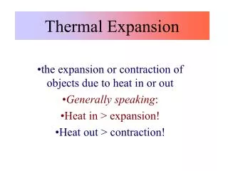
Radiation-Pressure and Thermal expansion • Kerr cavity: The intracavity power modifies the refraction index (then the optical • path) leading to changes in the intracavity power • Radiation-pressure driven cavity: The radiation pressure modifies the cavity length • the intracavity power changes the • radiation-pressure force varies • Photo-thermal expansion: Thermal expansion of the mirrors modifies the cavity • length the intracavity power changes the thermal • expansion varies Nonlinear dependence of the intracavity path on the optical power Multi-stability: cohexistence of stationary solutions
Physical Mechanism P P l l Interplay between radiation pressure and photothermal effect Optical injection on the long-wavelength side of the cavity resonance • The radiation pressure tends to increase the cavity lenght respect to the cold cavity value the intracavity optical power increases • The increased intracavity power slowly varies the temperature of mirrors heating induces a decrease of the cavity length through • thermal expansion
Physical Model L(t) = Lrp(t) + Lth(t) We write the cavity lenght variations as Radiation Pressure Effect Limit of small displacements Damped oscillator forced by the intracavity optical power Photothermal Effect Single-pole approximation The temperature relaxes towards equilibrium at a rate and Lth T Intracavity optical power Simple case: Adiabatic approximation The optical field instantaneously follows the cavity length variations
Physical model The stability domains and dynamics depends on the type of steady states bifurcations Stationary solutions Depending on the parameters the system can have either one or three fixed points
Bistability Analyzing the cubic equation for On this curve two new fixed points (one stable and the other unstable) are born in a saddle-node bifurcation 8 / 3 -8 / 3 Changes in the control parameters can produce abrupt jumps between the stable states
Bistability: Noise Effects Mode-hopping between the two stable states Noise Effects Resonance Out of Resonance Local stability region width 1 / Pin :critical for high power
Single solution: Hopf Bifurcation Single steady state solution: Stability Analysis They admit nontrivial solutions K et for eigenvalues given by Re = 0 ; Im = i Hopf Bifurcation: The steady state solution loses stability in correspondence of a critical value of 0 (other parameter are fixed) and a finite frequency limit cycle starts to grow
Hopf Bifurcation Boundary Frequency of the limit cycle Boundary of the bifurcation Q = 1, = 0.01, =4 Pin , =2.4 Pin For sufficiently high power the steady state solution loses stability in correspondence of a critical value of 0 Further incresing of 0 leads to the “inverse” bifurcation Linear stability analysis is valid in the vicinity of the bifurcations Far from the bifurcation ?
Relaxation oscillations small separation of the system evolution in two time scales: O(1) and O() We consider = 0 and 1/Q » is constant Fast Evolution Fixed Points () By linearization we find that the stability boundaries (F1,2) are given by C = -1
Relaxation oscillations Slow Evolution is slowly varying ( instantaneously follows variations) By means of the time-scale change = t and putting = 0 Defines the branches of slow motion (Slow manifold) Fixed point, p If () > p dt < 0 If () < p dt > 0 G=0 At the critical points F1,2 the system istantaneously jumps
Numerical Results Temporal evolution of the variable and corresponding phase-portrait as 0 is varied Q = 1 Far from resonance: Stationary behaviour In correspondence of 0c: Quasi-harmonic Hopf limit cycle Further change of 0: Relaxation oscillations, reverse sequence and a new stable steady state is reached
Numerical Results Temporal evolution of the variable (in the relaxation oscillations regime) and corresponding phase-portrait as Q is incresed Q > 1 Q= 5 Q=10 Q=20 Relaxation oscillations with damped oscillations when jumps between the stable branches of the slow manifold occurs
Numerical Results Q > 1 Three interacting time scales: O(1), O(1/Q), O() The competition between Hopf-frequency and damping frequency leads to a period-doubling route to chaos Between the self-oscillation regime and the stable state Chaotic spiking
Stability Domains: Oscillatory behaviour Stability domain in presence of the Hopf bifurcation Q » 1 For high Q is critical Stability domains for Q=1000, 10000,100000
Future Perspectives • Experiment on the interaction between radiation pressure and photothermal effect • Time Delay Effects (the time taken for the field to adjust to its equilibrium value) • Model of servo-loop control • Extend the model to the case of gravitational wave interferometers