Download
1 / 11
110 likes | 261 Vues
Tapering and prewhitening fFT. t aper, h(u). Need for prewhitening / prefiltering periodogram is generally biased. Smoothed periodogram. Expected value generally biased, but not for white noise. Improve by prefiltering Y filtered version of X with transfer function A

E N D
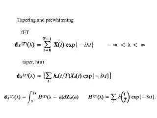
Tapering and prewhitening fFT taper, h(u)
Need for prewhitening/prefiltering periodogram is generally biased
Smoothed periodogram Expected value generally biased, but not for white noise
Improve by prefiltering Y filtered version of X with transfer function A dZY(λ) = A(λ)dZX(λ) fYY(λ) = |A (λ)|-2 fXX(λ) fXX(λ) = |A (λ)|-2fYY(λ) For example: detrend, “remove” peaks, fit autoregressive
The importance of prefiltering. The estimates are generally biased E{ fT()} = WT (-) f() d Seismic noise horizontal components recorded at UCB Estimated coherence can be 1,0 when no relation Estimated coherence can be 0.0 when linearly time invariantly related
postscript(file="seismic.eps") junkx<-scan("ts_drb.16.dat") junky<-scan("ts_drb.17.dat") par(mfrow=c(2,1)) xaxis<-c(1:2500)*.08 plot(xaxis,junkx,type="l",main="Vertical component seismic noise at Berkeley",xlab="time (sec)",ylab="",las=1) plot(xaxis,junky,type="l",main="West component",xlab="time(sec)",ylab="",las=1) par(mfrow=c(2,3)) junk<-spec.pgram(cbind(junkx,junky),spans=15,taper=0,detrend=F,demean=T,plot=F) junk$freq<-junk$freq/.08 plot(junk$freq,junk$spec[,1],type="l",las=1,main="Vertical noise",xlab="frequency (hertz)",log="y") plot(junk$freq,junk$spec[,2],type="l",las=1,main="West noise",log="y") plot(junk$freq,junk$coh,type="l",ylim=c(0,1),main="Raw data",las=1) abline(h=1-(1-.95)^(1/(.5*(junk$df-2))))
junkxx<-ar(junkx,order.max=2) junkyy<-ar(junky,order.max=2) Junkx<-junkxx$resid Junky<-junkyy$resid Junkx<-Junkx[3:length(Junkx)];Junky<-Junky[3:length(Junky)] Junk<-spec.pgram(cbind(Junkx,Junky),spans=15,taper=0,detrend=F,demean=T,plot=F) Junk$freq<-Junk$freq/.08 plot(Junk$freq,Junk$spec[,1],type="l",las=1,log="y") plot(Junk$freq,Junk$spec[,2],type="l",las=1,log="y") plot(Junk$freq,Junk$coh,type="l",ylim=c(0,1),main="AR(2) residuals",las=1) abline(h=1-(1-.95)^(1/(.5*(junk$df-2)))) graphics.off()