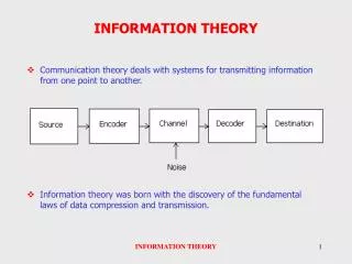
Chapter 6 Information Theory

1. Chapter 6Information Theory

2. 6.1 Mathematical models for information source • Discrete source

3. 6.1 Mathematical models for information source • Discrete memoryless source (DMS) Source outputs are independent random variables • Discrete stationary source • Source outputs are statistically dependent • Stationary: joint probabilities of and are identical for all shifts m • Characterized by joint PDF

4. 6.2 Measure of information • Entropy of random variable X • A measure of uncertainty or ambiguity in X • A measure of information that is required by knowledge of X, or information content of X per symbol • Unit: bits (log_2) or nats (log_e) per symbol • We define • Entropy depends on probabilities of X, not values of X

5. Shannon’s fundamental paper in 1948“A Mathematical Theory of Communication” Can we define a quantity which will measure how much information is “produced” by a process? He wants this measure to satisfy: • H should be continuous in • If all are equal, H should be monotonically increasing with n • If a choice can be broken down into two successive choices, the original H should be the weighted sum of the individual values of H

6. Shannon’s fundamental paper in 1948“A Mathematical Theory of Communication”

7. Shannon’s fundamental paper in 1948“A Mathematical Theory of Communication” The only H satisfying the three assumptions is of the form: K is a positive constant.

8. Binary entropy function H(p) H=0: no uncertainty H=1: most uncertainty 1 bit for binary information Probability p

9. Mutual information • Two discrete random variables: X and Y • Measures the information knowing either variables provides about the other • What if X and Y are fully independent or dependent?

11. Some properties Entropy is maximized when probabilities are equal

12. Joint and conditional entropy • Joint entropy • Conditional entropy of Y given X

13. Joint and conditional entropy • Chain rule for entropies • Therefore, • If Xiare iid

14. 6.3 Lossless coding of information source • Source sequence with length n n is assumed to be large • Without any source coding we need bits per symbol

15. Lossless source coding • Typical sequence • Number of occurrence of is roughly • When , any will be “typical” All typical sequences have the same probability

16. Lossless source coding • Typical sequence • Since typical sequences are almost certain to occur, for the source output it is sufficient to consider only these typical sequences • How many bits per symbol we need now? Number of typical sequences =

17. Lossless source coding Shannon’s First Theorem - Lossless Source Coding Let X denote a discrete memoryless source. There exists a lossless source code at rate R if bits per transmission

18. Lossless source coding For discrete stationary source…

19. Lossless source coding algorithms • Variable-length coding algorithm • Symbols with higher probability are assigned shorter code words • E.g. Huffman coding • Fixed-length coding algorithm E.g. Lempel-Ziv coding

20. Huffman coding algorithm P(x1) P(x2) P(x3) P(x4) P(x5) P(x6) P(x7) H(X)=2.11 R=2.21 bits per symbol

21. 6.5 Channel models and channel capacity • Channel models input sequence output sequence A channel is memoryless if

22. Binary symmetric channel (BSC) model Source data Output data Channel encoder Binary modulator Channel Demodulator and detector Channel decoder Composite discrete-input discrete output channel

23. Binary symmetric channel (BSC) model 1-p 0 0 p Input Output p 1 1 1-p

24. Discrete memoryless channel (DMC) {X} {Y} x0 y0 Input Output x1 y1 … … … xM-1 can be arranged in a matrix yQ-1

25. Discrete-input continuous-output channel If N is additive white Gaussian noise…

26. Discrete-time AWGN channel • Power constraint • For input sequence with large n

27. Source data Output data AWGN waveform channel • Assume channel has bandwidth W, with frequency response C(f)=1, [-W, +W] Channel encoder Modulator Physical channel Demodulator and detector Channel decoder Input waveform Output waveform

28. AWGN waveform channel • Power constraint

29. AWGN waveform channel • How to define probabilities that characterize the channel? Equivalent to 2W uses per second of a discrete-time channel

30. AWGN waveform channel • Power constraint becomes... • Hence,

31. Channel capacity • After source coding, we have binary sequency of length n • Channel causes probability of bit error p • When n->inf, the number of sequences that have np errors

32. Channel capacity • To reduce errors, we use a subset of all possible sequences • Information rate [bits per transmission] Capacity of binary channel

33. Channel capacity We cannot transmit more than 1 bit per channel use Channel encoder: add redundancy 2ndifferent binary sequencies of length n contain information We use 2m different binary sequencies of length m for transmission

34. Channel capacity • Capacity for abitray discrete memoryless channel • Maximize mutual information between input and output, over all • Shannon’s Second Theorem – noisy channel coding • R < C, reliable communication is possible • R > C, reliable communication is impossible

35. Channel capacity For binary symmetric channel

36. Channel capacity Discrete-time AWGN channel with an input power constraint For large n,

37. Channel capacity Discrete-time AWGN channel with an input power constraint Maximum number of symbols to transmit Transmission rate Can be obtained by directly maximizing I(X;Y), subject to power constraint

38. Channel capacity Band-limited waveform AWGN channel with input power constraint - Equivalent to 2W use per second of discrete-time channel bits/channel use bits/s

39. Channel capacity

40. Channel capacity • Bandwidth efficiency • Relation of bandwidth efficiency and power efficiency