A brief Introduction to Automated Theorem Proving
570 likes | 946 Vues
A brief Introduction to Automated Theorem Proving. Theoretical Foundations, History and the Resolution Calculus for classical First-order Logic Uwe Keller based on material by B. Beckert, R. Hähnle, A. Voronkov, A. Leitsch and T. Tammet. Content. Intoduction Motivation & History

A brief Introduction to Automated Theorem Proving
E N D
Presentation Transcript
A brief Introduction to Automated Theorem Proving Theoretical Foundations, History and the Resolution Calculus for classical First-order Logic Uwe Keller based on material by B. Beckert, R. Hähnle, A. Voronkov, A. Leitsch and T. Tammet
Content • Intoduction • Motivation & History • Theorem Proving, ATP and Calculi • Foundations • FOL, Normalforms & Preprocessing, Metaresults • Resolution • Basic calculus, Unification • Refinements, Redundancy • Decision procedures • Chain Resolution • A Variant of Resolution for the Semantic Web • Demo
Part I:Introduction Motivation & History Theorem Proving, ATP and Calculi
(automated) Deduction Modelling Logic and Theorem Proving Real-world description in natural language. Mathematical Problems Program + Specification Formalization Syntax (formal language). First-order Logic, Dynamic Logic, … Semantics (truth function) Calculus (derivation / proof) Correctness Valid Formulae Provable Formulae Completeness
How did it start … • Results from first-half of the 20th century in mathematical logic showed … • we can do logical reasoning with a limited set of simple (computable) rules in restricted formal languages like First-order Logic (FOL) • That means computers can do reasoning! • Implementation of ATP • First: Computers where needed :- ) • AI as a prominent field: Reasoning as a basic skill! • Mid 1950‘s first attempts to implement an ATP • Today • (A)TP is no longer only a part of main stream AI • Central shared problem: How to represent and search extremely large search spaces!
A rough timeline in ATP … • before 1950: Proof-theoretic Work by Skolem, Herbrand, Gentzen and Schütte • 1954: First machine-generated Proof (Davis) • 1955ff: Semantic Tableaus (Beth, Hinitkka) • 1957: First machine-generated Proof in Logic Calculus (Newell & Simon) • 1957: Lazy substitution by free (dummy) Vars (Kanger, Prawitz) • 1958: First prover for Predicate Logic (Prawitz) • 1959: More provers (Gilmore, Wang) • 1960: Davis-Putnam Procedure (Davis, Putnam, Longman) • 1963: Unification (J.A. Robinson) • 1963ff: Resolution (J.A. Robinson); Inverse Method (Maslov) • 1963ff: Modern Tableau Method (Smullyan, Lis) without Unification • 1968: Modelelimination (Loveland), with Unification • 1970ff: PROLOG (Colmerauer, Kowalski), Refinements of Resolution • 1971: Connection Method (Bibel), Matings (Andrews) with Unification • 1985: ATP in non-classical logics, Renaissance of Tableaux Methods • 1987: Tableaus with Unification • 1993ff: Renewed interest in Instance-based Methods: DPLL, Modelevolution • …
Theorem Proving • Given • a formal language (or logic) L • a calculus C for this language (= set of rules) • a conjecture S and a set of assumptions or axioms A in the language L • Determine • Can we construct a proof for S (from A) in calculus C? • Logic = Syntax + Semantics + Calculus • TP = Proof-search in C (Huge search problem) • Correctness and completeness of Calculi essential properties • Calculus = Non-deterministic Algorithm • Central problem in ATP: How to implement a non-deterministic algorithm „efficiently“ on a deterministic machine :- )
Theorem Proving (II) • Research areas • Interactive / tactic TP vs. Automated TP • Classical Logic vs. Non-classical logics • Calculi for … • ATP - General principle: Refutation approach • Resolution, Tableau, Inverse Method, Instance-based Methods • ITP – General principle: Show Proof situation/context • Sequent Calculi • others – General principle: Generation of complex formulae based on very simple axioms • Hilbert-style Calculi • Central difference: • What are the elements in a proof & what is a proof?
Main TP Applications • Main Applications • Software & Hardware Verification • Theorem proving in Mathematics • Query answering in rich knowledge bases (Ontologies) • Verification of cryptographic protocols • Retrieval of Software Components • Reasoning in non-classical Logics • Program synthesis … • … many systems implemented • ATP: Vampire, Otter, Spass, E-SETHEO, Darwin, Epilog, SNARK, Gandalf … • ITP: Isabelle/HOL, Coq, Theorema, KeY-Prover …
Why is FOL of special interest in the ATP community ? • There are less & more expressive logics than FOL • Classical Propositional Logic, Modal Propositional Logic, Description Logics, Temporal Propositional Logic • Higher-order Predicate Logics, Dynamic Predicate Logics, Type Theory • Research in ATP mainly focused on FOL • FOL is very expressive, many real-world problems can be formalized in FOL • FOL turned out to be the most expressive logic that one can adequately approach with ATP techniques
Example … • Theorem in (elementary) Calculus • Nullstellensatz: Every function which is continous over a closed interval I=[a,b] must take the value 0 somewhere in I if f(a) <= 0 and f(b) >= 0 • Proof idea: Consider the Supremum l of set M = {x : f(x) <= 0, a<=x<=b} and show that f(l) = 0
Example (II) … • Formalization • Compact (only LEQ) • Redundancy-free • Specific definitions • Continous functions • Main idea of proofis already encoded • Use Supremum • Can be done by anATP system • … but without properFormalization ?!? • ATP better than humanprover? Robbins Problem in Algebra • Intelligent Proving vs.Combinatorical proving
Part II:Foundations FOL, Normalforms & Preprocessing, Metaresults
Classical First-order Logic (FOL) • Syntax • Signature § • Function Symbols, Predicate Symbols, Arity, logical Connectives, Quantors • Terms (over §), Atomic Formulae (over §), Formluae (over §) • Definition relative to the signature § of the predicate logic • Semantics • First-order structure / interpretation S = (U,I) • Universe U + Signature-Interpretation I • Constants I(c) = element of U • Functionsymbols I(f) = total functions on U • Relationsymbols I(R) = relation on U • Logical connectives and quantors in the usual way • Definition relative to the signature § of the predicate logic
Classical FOL (II) • Model of a statement • An interpretation S = (U,I) is called a model of a statement s iff valS(s) = t • What does it mean to infer a statement from given premisses? • Informally: Whenever our premisses P hold it is the case that the statement holds as well • Formally: Logical Entailment • For every interpretation S which is a model of P it holds that S is a model of S as well • Special case: Validity – Set of premisses is empty • Logical entailment in a logic L is the (semantic) relation that a calculus C aims at formalizing syntactically (by means of a derivability relation)! • Logical entailment considers semantics (Interpretations) relative to a set of premisses or axioms!
Normal Forms • What is a normal form? • Why are they interesting? • Relation to ATP? • Conversion of input to a specifc NF my be required by a calculus (e.g. Resolution) )Preprocessing step • ATP in a sense can be seen as a conversion in a NF itself, borderline is fuzzy in a sense • Normalforms in FOL • Negation Normal Form • Standard Form • Prenex Normal Form • Clause Normal Form (in a sense a „logic free“ form) • There are logics where certain NF do not exist, like CNF in a Dynamic First-order Logic • Certain calculi then can not be applied in these logics!
Negation Normal Form • A formula is in Negation NF (NNF) iff. it contains no implication and no bi-implication symbols and all negation symbols occur only as part of a literal (directly in front of atomic formulae) • How to achieve this NF ? • Replace implication and bi-implication by their definition (in terms of Æ and Ç) • Move negation symbols inside to atomic formulae • De Morgan laws • Dualize quantifiers when moving negation symbols over a quantor • Eliminate multiple negations • All these syntactical transformations generate semantically equivalent formulae • Example
Standard Form • A formula A is in Standard Form if no variable x in A occurs both bound and free and no bound variable is used as a quantor variable for multiple subformulae • How to generate this NF? • Bounded renaming of quantor variables and the respective occurrences • Transformed formulae is semantically equivalent to original one • Example (8 x P(x) Æ Q(z)) ! (9 x R(x) Ç9 z (P(z) Æ Q(z)))
Prenex Normal Form • A formula A is in Prenex NF iff. it is of the form A = Q1x1 … Qnxn B where Qk is a universal or existential quantor and B contains no quantors. B is called the Matrix of A • How to construct this NF? • Transform A in NNF and Standard Form • Move iteratively outermost quantor to the outside until it reaches another quantor. Quantors may not cross quantors of different sort (in-scope relation between quantor occurrences may not be changed) • This transformation generates a formulae which is logically equivalent to the original one. • Example
Clause Normal Form • A formula A is in Clause NF iff. it is in PNF, closed, the prefix only contains universal quantors and the Matrix is on conjunctive normal form. • In other words: A = 8 x1 … 8 xn ( (L1,1Ç … Ç L1,m1) Æ … Æ (Lk,1Ç … Ç Lk,mk)) where Li,j is a literal (negated or positive atomic formula) • How to construct this NF? • Transform A in NNF and Standard Form • Transform result in PNF • Remove existential quantors by Skolemization (Function terms) • Apply Distributivity laws to convert Matrix of the result in conjuntive normal form (conjunction of discjunction of literals) • This transformation results in a formula which is not logically equivalent, but it is satisfiability-preserving (which is enough for the ATP methods later) • Example
Clause Normal Form (II) • A formula A is in Clause NF can be written as A = 8 x1 … 8 xn ( (L1,1Ç … Ç L1,m1) Æ … Æ (Lk,1Ç … Ç Lk,mk)) where Li,j is a literal (negated or positive atomic formula) • Since every formula can be transformed into CNF, the CNF can be seen as „logic free“ representation of a formulae • All quantors are universal, no free variables are allowed -> drop quantors • Matrix is in CNF = Conjunction of Disjunction of Literals -> Model as a Set of Sets of Literals • Example • The sketched transformation to CNF is not optimal • Exponential blowup possible (already for NNF) • Syntactical structure of the original formula gets lost • Skolemsymbols have unnecessarily many parameters • Unnecessarily many new skolem systems are introduced • One can improve all these aspects of a transformation to CNF! • Skolemization before PNF transformation, Definitorial CNF for Matrix, Reuse of Skolem functions
Metaresults • Metaresult = Property of a Logic L • Most famous example: Gödels Incompleteness Theorems! • Here some metaresults for FOL which form the theoretical foundation of ATP • carry over to many other logics as well • Deduction Theorem • If M [ s ² s‘ then M ² s‘ ! s • Logical entailment can be reduced to validity • Proof by contradiction • If M is a set of closed formulae thenM ² s iff. M [ {¬s} is unsatisfiable (i.e. has no model) • Logical entailment can be reduced to unsatisfiability checking • Refutation can be used as a universal principle for inference in FOL
Metaresults (II) • Complexity of logical entailment, validity and satisfiability • Propositional Logic • Logical entailment (²-relation) is decidable, Satisfiability too • Set of valid formulae is co-NP-complete • Set of satisfiable formulae is NP-complete • First-order Predicate Logic • Logical entailment / validity / satisfiability is undecidable • Set of valid formulae is semi-decidable (recursively enumerable) • Set of satisfiable formulae is not recursively enumerable
Metaresults (III) • Term Interpretations and Herbrand Theorem • S = (U,I) is term-interpretation if U = Term0 • Let Term0 be non-empty. An interpretation S = (U,I) is called Herbrand-Interpretation if • S is term-interpretation and • I(f)(t1,…,tn) = f(t1,…,tn) for all n-ary function symbols f 2 and ground terms t1,…,tn • Herbrand-Modell of s is Herbrand-Intp. I with I ² s • Herbrand-Interpretations are special because they have a simple universe (syntactical) and Terms are basically uninterpreted. Quantifiers then have ground terms as their range! • Computers can deal with such special (syntactical) interpretations, but not with interpretations in general!
Metaresults (IV) • Term Interpretations and Herbrand Theorem • Let M be a set of closed formulae s in Prenex-Normalform that contain no existential quantors (for instance s in CNF) • Let T be a set of terms (over signature ) • T(M) := set of T-instances of M, i.e. replace every occurence of a (universal) variable in any formulae in M with any term in T • Herbrand Theorem • Let Term0 be non-empty and M a set of formulae in Prenex-NF without existential quantors. • Then the following statements are equivalent • M has a model • M has a Herbrand-model • Term0(M) has a model • The last set is a set of formulae in propositional logic
Metaresults (V) • Compactness of FOL • A (possibly infinite) set M of formulae has a model iff every finite subset M‘ ½ M has a model (i.e. is satisfiable) • Combining Compactness with Herbrand‘s Theorem • Let Term0 be non-empty and M a set of formulae in Prenex-NF without existential quantors. • Then M is unsatisfiable iff. T(M) is unsatisfiable for a finite set of ground terms T ½ Term0 • Note that T is a finite set of ground terms over the signature of the formula set M • No „external“ functions symbols have to be considered! • Allows for using guided substitutions (Unification!)
Metaresults (VI) • That means: logical entailment / validity can be checked • by reduction to unsatisfiabiliy of a set of formulae M‘ • which can done by finding suitable finite (counter)-examples for the quantfied variables such that a contradiction arises • One can only use the Signature of the given set M‘ to find the counterexamples • Basically this is what all ATP procedures do: Find a finite set of counterexamples (objects) such that a respective instance of the orginial formula set is determined as being inconsistent (unsatisfiable) • The theorem immediately gives an algorithm for ATP! • Problem: How to construct / find T in the theorem in a clever way?
Herband‘s Theorem:From Clause Logic to Propositional Logic Clauses Clause Logic (Ground) Substitutions Incons- istent set Ground clauses Propositional Logic
Part III:The Resolution Calculus Pre-resolution phase: Gilmore‘s Methods, Davis-Putnam Procedure Unification Basic Resolution Calculus Refinements, Redundancy
Pre-Resolution period: Gilmore‘s Method • First ATP procedure for First-order logic • Directly based on Herbrands Theorem • Reduction of FOL entailment to satisfiability in Prop. Logic • How to generate candidates C‘ for propositional satisiability checking from a FOL clause set C • Saturation by ground instances from Hn(C) (= set of ground terms of depth · n) • More precisely: Successively generate the sets C‘n of ground clauses := {c : c 2 C and rg() µ Hn(C) } • Since H_n( C) grow exponentially it is very important to have a good algorithm for checking satisfiability
Pre-Resolution period: Gilmore‘s Method • „Easy“ test of satisfiability of the generated C‘ set of ground clauses: • Transform C‘ into Disjunctive Normal Form • D = DNF(C‘) is unsatisfiable iff every consitutent of D contains a contradiction L ƬL for some literal L • Can be done in deterministic time O(n log(n)) • Problem: Convertion from CNF into DNF (almost always) exponential (inherently complex, since otherwise P = NP), (not known at that time!) • Pseudocode begin contr := false while not contr do D‘ := DNF(C‘_n) contr := all constitutents of D‘ contain complementary literals n:=n+1 end while end
Pre-Resolution period: Gilmore‘s Method • Weak points of Gilmore‘s approach … • The generation of the candidate ground clause sets C‘n to be checked • the discjunctive normal form transfomation • First weakness is inherent to all procedures directly applying Herbrands theorem • The second problem concerns propositional logic only • Gilmore‘s pioneering implementation did not yield actual proofs for quite simple predicate logic formulas • A possible improvement • Avoid transformation to DNF and try to find „good“ decision methods for satisfiability on CNFs • This is basically what was achieved by Davis and Putnam [DP,1960] shortly after Gilmore‘s implementation
Pre-Resolution period:Davis-Putnam Procedure • Like Gilmore‘s method based on successive production of ground caluse sets C‘N and testing of their unsatisfiability • (Still) very efficient decision method for satisfiability. Requires CNF for ground clauses. • Invented originally for FOL, it became the most powerful SAT decision procedure for Propositional Logic. Many very powerful SAT solvers still are refining DPP today. • Davis-Logemann-Loveland Rules [DLL, 1962] • Preliminary step: Reduce all clauses in C • Eliminate multiple occurrences of the same literal (leave only one). Generates a clause set C‘ • Then apply the follwing rules non-deterministically to C‘ • Tautology-Rule • One-Literal-Rule • Pure-Literal-Rule • Splitting-Rule
Pre-Resolution period:Davis-Putnam Procedure • Davis-Logemann-Loveland Rules [DLL, 1962] • Tautology-Rule: Delete all clauses in C‘ containing complementary literals • One-Literal-Rule: If there is a clauses c = {l} with only one literal l, remove all clauses d from C‘ which contain l, and remove the dual literal ld from all other clauses • Pure-Literal-Rule: Let D‘ µ C‘ with the following property: There exists a literal l appearing in all clauses of D‘, but ld does not appear in C‘. Then delete D‘ from C‘ • Splitting-Rule: Let C‘ = {A1,…,An,B1,…,Bm} [ R such that R contains l nor ld, all Ai contain l but not ld and all Bj contain ld but not l. Let A‘i = Ai after deletion of l and let B‘j = Bj after deletion of ld.Then split C‘ into C‘1 = {A‘1,…,A‘n} [ R and C‘2={B‘1,…,B‘m} [ R • Properties of the DLL procedure • The rules are essentially reductive (atoms are in each step deleted) • The rules are correct (rules preserve satisfiability; in case of split only for one of the new introduced clauses sets • The procedure generates sets that contain the empty clause for all cases (of the applied splits) iff C‘ is unsatisfiable (decision criteria: correctness and completeness, termination) Example: C = {P Ç Q, R Ç S Ç S, ¬R Ç S, R Ç ¬S, ¬R Ç ¬S, P Ç ¬Q Ç ¬P}
Pre-Resolution period:Davis-Putnam Procedure • Pseudocode of the First-order ATP procedure by Davis & Putnam begin {C finite set of clauses} if C does not contain („real“) function symbols then apply DP1 – DP3 to C‘_0; check the DP decision tree for unsatisfiability else begin n:= 0; contr := false while not contr do perform DP1 – DP3 on C‘_n if the DP-decision tree proves unsatisfiability then contr := true else contr := false n:=n+1 end while end end • Nondeterministic (DP3) • If C does not contain function symbols (with arity > 0) then the procedure always terminates (== decision procedure for FOL clause set) • If C is satisfiable and C contains function symbols then the algorithm does not terminate • Yields a decision procedure for validity of the Bernays-Schönfinkel class in FOL (8*9*) DP1: Reduce all clauses DP2: Delete all tautologies DP3: Construct a DP decision tree according to the given rules
Interlude:Inferences & Inference systems • An inference I has the formwhere n ¸ 0, F1,…,Fn, G are formulae • An inference rule R is a set of inferences • more precisely a decidable (usually efficiently computable) n+1-ary relation over formuale • Usually one uses schematic variables for representing formulae in inference rules and attach some (most often syntactic) conditions to these variables • Every instance I 2 R is called an instance of R • An inference system§ is a (finite) set of inference rules • A proof of G from P in § is a finite sequence of formulae F1, … Fn such that • Fn = F and • for all Fi (i · n) it holds that either Fi2 N or there is an inference I such that Fi is the conclusion of I and all the premisses P1, … Pj of I are contained in the prefix F1, …, F(i-1) • Here we mainly consider inference systems on clauses, for instance Resolution F1 F2 … Fn G Premisses Conclusion
A Revolution in ATP: Robinson‘s Resolution Principle • In some sense the simplest possible calculus for FOL (without equality) • In principle only a single inference rule which combines substution and atomic cut • Possible since it requires set of input formulae in CNF (very simple and uniform syntactic form) • Binary substitution rule computing a „minimal“ substitution which makes two atoms equal • A quote from Robinsons landmarking paper [Robinson, 1965] … • Theorem-proving on the computer, using procedures based on the fundamental theorem of Herbrand concerning the FOL Predicate Calculus, is examined with a view towards improving the efficiency and widening the range of practical applicability of these procedures. A close analysis of the process of substitution (of terms for variables) and the process of truth-functional analysis of the results of such substitutions reveals that both processes can be combined into a single new iterating process (called resolution)which is vastly more efficient than the older cylcic procedures consisting of substitution stages alternating with truth-functional analysis stages.
A Revolution in ATP: Robinson‘s Resolution Principle • The basic Resolution Calculus (BRC) • Ground case • General case • Fundamental aspects: • Iterative grounding of the clause set • „Guided“ guessing of interesting instances (Unification) built into the calculus • Resolving upon an atom L does not require L to be ground (unnecessary grounding avoided) Binary Resolution L Ç C ¬L Ç D C Ç D C Ç L Ç L C Ç L Factoring Binary Resolution L Ç C ¬L‘ Ç D (C Ç D) C Ç L Ç L‘ (C Ç L) Factoring where is the most general unifier of L and L‘
Basic Resolution Calculus:Properties • Properties of the basic Resolution Calculus • Given any two clauses, there are only finitely many resolvents using the Resolution Inference Rule. • The Resolution Calculus is sound • If c is provable from C in BRC then C ² c • This means in particular: If we can derive the emtpy clause then C is unsatisfiable • The Resolution Calculus is refutationally complete • A set C of clauses is unsatisfiable then the empty clause can be proven (derived) from C • Altogether • A set C of clauses is unsatisfiable iff. there is a proof for the empty clause from C in BRC • Remark: Soundness of the inference system can be relaxed to satisfiability- preserving! • How to find a contradiction (empty clause) starting with an initial (unsatisfiable) formula set? • Saturation approach (wrt. the inference system BRC)
Resolution:Proof search by Saturation • Saturated sets • A set of clauses C is called saturated (wrt. inference system ) if every inference in with premises in C gives a clause in C • Completness reformulated (in terms of saturated sets) • A set C of clauses is unsatisfiable iff every saturated set S of clauses with C µ S also contains the empty clause • That means: Simply construct a(ny) saturated set S of clauses (wrt. BRC) S (saturation algorithm) • Simple algorithm • S:= set of input clauses • while not finished do • Repeatedly apply all inferences to clauses in S, adding to S conclusions of these inferences • If the empty clause is proved, terminate with success. If no inference rule is applicable, terminate with failure
Goal clause candidate clause given clause Search space Search space Resolution:Proof search by Saturation Conclusions
Search space Resolution:Proof search by Saturation • Most likely scenario ….
Resolution:Proof search by Saturation • Possible theoretical scenarios • At some moment the empty clause is generated, in this case the input set of clauses is unsatisfiable • Saturation will terminate without ever generating the empty clause, in this case the input set of clauses is satisfiable • Saturation will run forever, but without generating the empty clause. In this case the input set of clauses is satisfiable • Possible practical scenarios • At some moment the empty clause is generated, in this case the input set of clauses is unsatisfiable • Saturation will terminate without ever generating the empty clause, in this case the input set of clauses is satisfiable • Saturation will run until we run out of resources, but without generating the empty clause. In this case it is unknown whether the input set of clauses is (un)satisfiable
Resolution:How to saturate in clever way ? • The simple saturation algorithm is highly inefficient • Apply inferences not in an arbitrary way, but within some senseful / useful order. • Generate the empty clause as early as possible in the saturation process • „Prefer“ some inferences over others (in a sense), for instance goal directedness • Actually what we need to ensure then to have completness guaranteed is fairness: • A saturation algorithm is fair iff every possible inference is eventually selected • Completness Theorem reformulated (for Saturation Algorithms) • Let A be a fair saturation algorithm. A set C of clauses is unsatisfiable iff A eventually produces the empty clause • Central problem: How to find „good“ saturation algorithms!