Lecture 1: Simple Keynesian Model

Lecture 1:Simple Keynesian Model National Income Determination Two-Sector National Income Model

Outline • Introduction • Preliminaries definitions and concepts • National Income Determination Model OR Simple Keynesian Model • Consumption Function • Investment Function • National Income Identities • Expenditure Function • Equilibrium condition

Macroeconomics • Recall that the study of macroeconomics focuses on a set of issues and goals: • National income, general price level and inflation rate, unemployment rate, interest rate and the exchange rate

Macroeconomics • What is GDP? • Rising long term trend in GDP ensures continuous growth • However, short term characterized by oscillations. • Why does GDP behave as it does? • Rising in some periods and falling in others? • What can governments do to influence it? • To answer, we need a theory of national income • i.e. a theory that explains the size of and changes in national income

Key Concepts • Expenditure flows • Expenditure flows are real (not nominal) flows • i.e. measured in constant prices because we are concerned with real changes • All expenditure flows are planned (or desired) flows • i.e. what people intend to spend, and not what they actually spend • All expenditure flows are aggregate flows • We are not concerned with the behaviour of individual households or firms

Basic Assumptions • Potential national income is constant • An economy’s productive capacity changes slowly from year to year • There are unemployed supplies of all factors of production • i.e. output can be increased by increasing use of unemployed land, labouror capital, without bidding up prices • The interest rate and general price level are constant • Assumption relaxed in later studies • There are only households and firms (2-sector). • No government and foreign trade

Recap: Circular Flow Model • Underlying assumptions? • Only two economic units and only two markets • Households own all factors of production • Households spend all their resources in the market for goods and services

The Circular Flow of Income • This refers to the flow of expenditures on output and factor services passing between domestic firms and households • Any other flow that is not a part of this model is either an injection or a withdrawal/ leakage • Injection • Income received, either by households or firms, that does not arise from the spending of the other group • Withdrawal • Income received, either by households or firms, that is not passed on to the other group by buying goods or services from it

The Circular Flow of Income • Only domestic households and firms • Economy produces only 2 kinds of commodities • Consumer goods- produced by firms and sold to households • Investment goods- produced by firms and sold to other firms that use them

The Basic Model:The Effects of Savings and Investments • Households receive income from firms and pass back through consumption expenditure • Savings is income received by households that they do not pass back • Savings an injection or withdrawal? • Exerts a contractionary force on the flow of income • Investments expenditure creates incomes for the firms that produce capital goods and for the factors they employ • This income does not arise from household expenditures • Investment expenditures injection into the economy or a withdrawal? • Exerts an expansionary force on the flow of income

Definitions • Given assumptions, total output wholly dependent on total demand • Not supply since we assume unemployed factors • Total demand comprises • Desired consumption expenditure, C • Desired investment expenditure, I • Aggregate desired expenditure refers to total amount of purchases that all spending units (firms and households) within the economy wish to make • i.e. E= C + I

Behavioural Assumptions about C and I • Autonomous vs Induced expenditures • Autonomous/ exogenous- expenditure flows that are not influenced by any variable the theory is designed to explain • Theory explains variations in national income so any expenditure that does not vary with national income is exogenous • Also called constants. Can change, but not for reasons explained by the national income theory

Behavioural Assumptions about C and I • Autonomous vs Induced expenditures • Induced/ endogenous expenditures- any expenditure that is related to national income • Variations in these expenditure flows are induced by changes in national income

Behavioural Assumptions about C and I • The Investment, I, component • For now, we assume investment fixed • Firms plan to spend a constant amount on plants and equipment each year • Firms plan to hold their inventories constant • Planned housing construction is constant from year to year • Investment is therefore an autonomous/ exogenous expenditure flow • i.e. I= I* • Graphical Illustration

Investment Function:Graphical Illustration Investment expenditure I = I* Real National Income

Behavioural Assumptions about C and I • The Consumption, C, component • Consumption is a function of national income • We assume that consumption is always a constant fraction of national income • i.e. C= cY, 0<c<1 • Where c is the fraction of income spent on consumption • Households also decide how much of their income to consume and save • i.e. S= sY, 0<s<1 and s= 1-c • Where s is the fraction of income saved • Graphical Illustration of consumption function

Consumption Function: Graphical Illustration Consumption expenditure Consumption expenditure C = cY C = C’ Real National Income Real National Income

Consumption Functions • We know that C= cY • What happens if c  ? • What happens if Y  ? • But what exactly is c?

Propensities to Consume and Save • Consumption propensities summarize the relationship between consumption and income

Consumption Function • Marginal Propensity to Consume MPC = c • It is defined as the change in consumption per unit change in income • It is the proportion of each new increment of income that is spent on consumption • C= cY • MPC = C / Y • Average Propensity to Consume APC= c • It is defined as the ratio of total consumption C to total income Y • It is the average amount of all income spent on consumption • APC = C / Y

Consumption Function • Relationship between APC and MPC • C = cY • Divide by Y to obtain APC • C/Y = c • Differentiate by Y to obtain MPC • C / Y = c • Therefore, when C= cY, APC = MPC = c

National Income Identities • An identity is true for all values of the variables • In a 2-sector economy, expenditure consists of spending either on consumption goods C OR investment goods I. • Aggregate expenditure (AE OR E) is ,by definition, equal to C plus I • E  C + I

National Income Identities • National income Y received by households, by definition, is either saved S OR consumed C. • Y C + S

National Income Identities • In equilibrium, aggregate expenditure E is, by definition, equal to national income Y • Y  E (output- expenditure approach) • C + S  C + I •  S  I (withdrawals- injections approach)

Equilibrium Income • Equilibrium is a state in which there is no internal tendency to change. • It happens when • firms and households are just willing to purchase everything produced Y = E (v.s. Micro: Qs = Qd) • This is the Income-Expenditure Approach • planned saving is equal to planned investment S = I • This is the Injection-Withdrawal Approach

Equilibrium Income • Y > E  Excess supply • planned output > planned expenditure  • unexpected accumulation of stocks OR • unintended inventory investment OR • involuntary increase in inventories • Firms will reduce output

Equilibrium Income • Y < E  Excess Demand • planned output < planned expenditure  • unexpected fall in stocks OR • unintended inventory dis-investment OR • involuntary decrease in inventories • Firms will increase output

Equilibrium Income • Y= E  Equilibrium • There is no unintended inventory investment OR dis-investment • Y=E

Equilibrium Income: Summary • When there is excess supply, i.e., planned output > planned expenditure, firms will reduce output to restore equilibrium • When there is excess demand, i.e., planned expenditure > planned output, firms will increase output to restore equilibrium

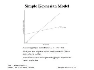
Aggregate Expenditure Function • Aggregate expenditure is comprised of consumption, C, and Investment, I i.e. E = C + I • Using functional forms, • C = cY and I = I* •  E = I* + cY • Graphical representation

Aggregate Expenditure Function:Graphical Illustration Slope of tangent = c C, I, E I C Slope of tangent=0 Y I = I* C = cY E = I*+ cY

Readings • Lipsey and Chrystal • Pp: 467- 480

Next Class • Output-Expenditure Approach to Income Determination • Expenditure Multiplier • Saving Function • Injection-Withdrawal Approach to Income Determination • Paradox of Thrift

Lecture 1: Simple Keynesian Model