Establish retention probabilities

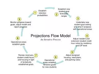
1. Establish new student goal forecasts/ ranges Establish retention probabilities 1 2 3 9 Monitor progress toward goals, adjust model and report progress Undertake new student goal setting and what if analyses with operational areas Projections Flow Model An Iterative Process 4 8 Adjust resident and extension student credit hour ratios by residency and CIP level Operational areas establish goals 5 Review revenues, student credit hours, and housing in light of tentatively established goals 7 Adjust assigned housing, meal plans, and parking ratios 6 Operational areas establish tentative goals for new students

2. 1 Establish retention probabilities

3. Establish new student goal forecasts/ ranges Establish retention probabilities 1 2 3 9 Monitor progress toward goals, adjust model and report progress Undertake new student goal setting and what if analyses with operational areas Projections Flow Model An Iterative Process 4 8 Adjust resident and extension student credit hour ratios by residency and CIP level Operational areas establish goals 5 Review revenues, student credit hours, and housing in light of tentatively established goals 7 Adjust assigned housing, meal plans, and parking ratios 6 Operational areas establish tentative goals for new students

4. 2 Establish new student goal forecasts/ranges

5. Establish new student goal forecasts/ ranges Establish retention probabilities 1 2 3 9 Undertake new student goal setting and what if analyses with operational areas Monitor progress toward goals, adjust model and report progress Projections Flow Model An Iterative Process 4 8 Adjust resident and extension student credit hour ratios by residency and CIP level Operational areas establish goals 5 Review revenues, student credit hours, and housing in light of tentatively established goals 7 Adjust assigned housing, meal plans, and parking ratios 6 Operational areas establish tentative goals for new students

6. 3 Undertake new student goal setting and what if analyses with operational areas

7. Undertake new student goal setting and what if analyses with operational areas Establish new student goal forecasts/ ranges Establish retention probabilities 1 2 3 9 Monitor progress toward goals, adjust model and report progress Projections Flow Model An Iterative Process 4 8 Adjust resident and extension student credit hour ratios by residency and CIP level Operational areas establish goals 5 Review revenues, student credit hours, and housing in light of tentatively established goals 7 Adjust assigned housing, meal plans, and parking ratios 6 Operational areas establish tentative goals for new students

8. 4 Adjust resident and extension student credit hour ratios by residency and CIP level

9. Undertake new student goal setting and what if analyses with operational areas Establish new student goal forecasts/ ranges Establish retention probabilities 1 2 3 9 Monitor progress toward goals, adjust model and report progress Projections Flow Model An Iterative Process 4 8 Adjust resident and extension student credit hour ratios by residency and CIP level Operational areas establish goals 5 Review revenues, student credit hours, and housing in light of tentatively established goals 7 Adjust assigned housing, meal plans, and parking ratios 6 Operational areas establish tentative goals for new students

10. 5 Adjust assigned housing, meal plans, and parking ratios

11. Undertake new student goal setting and what if analyses with operational areas Establish new student goal forecasts/ ranges Establish retention probabilities 1 2 3 9 Monitor progress toward goals, adjust model and report progress Projections Flow Model An Iterative Process 4 8 Adjust resident and extension student credit hour ratios by residency and CIP level Operational areas establish goals 5 Review revenues, student credit hours, and housing in light of tentatively established goals 7 Adjust assigned housing, meal plans, and parking ratios 6 Operational areas establish tentative goals for new students

12. 6 Operational areas establish tentative goals for new students

13. Undertake new student goal setting and what if analyses with operational areas Establish new student goal forecasts/ ranges Establish retention probabilities 1 2 3 9 Monitor progress toward goals, adjust model and report progress Projections Flow Model An Iterative Process 4 8 Adjust resident and extension student credit hour ratios by residency and CIP level Operational areas establish goals 5 7 Review revenues, student credit hours, and housing in light of tentatively established goals Adjust assigned housing, meal plans, and parking ratios 6 Operational areas establish tentative goals for new students

14. 7 Review revenues, student credit hours, and housing in light of tentatively established goals

15. Undertake new student goal setting and what if analyses with operational areas Establish new student goal forecasts/ ranges Establish retention probabilities 1 2 3 9 Monitor progress toward goals, adjust model and report progress Projections Flow Model An Iterative Process 4 8 Adjust resident and extension student credit hour ratios by residency and CIP level Operational areas establish goals 5 7 Review revenues, student credit hours, and housing in light of tentatively established goals Adjust assigned housing, meal plans, and parking ratios 6 Operational areas establish tentative goals for new students

16. 8 Operational areas establish goals

17. Establish new student goal forecasts/ ranges Establish retention probabilities 1 2 3 9 Undertake new student goal setting and what if analyses with operational areas Monitor progress toward goals, adjust model and report progress Projections Flow Model An Iterative Process 4 8 Adjust resident and extension student credit hour ratios by residency and CIP level Operational areas establish goals 5 7 Review revenues, student credit hours, and housing in light of tentatively established goals Adjust assigned housing, meal plans, and parking ratios 6 Operational areas establish tentative goals for new students

18. 9 Monitor progress toward goals, adjust model and report progress

19. Establish new student goal forecasts/ ranges Establish retention probabilities 1 2 3 9 Undertake new student goal setting and what if analyses with operational areas Monitor progress toward goals, adjust model and report progress Projections Flow Model An Iterative Process 4 8 Adjust resident and extension student credit hour ratios by residency and CIP level Operational areas establish goals 5 Review revenues, student credit hours, and housing in light of tentatively established goals 7 Adjust assigned housing, meal plans, and parking ratios 6 Operational areas establish tentative goals for new students

20. Time Series and Forecasting • Time-series data describes the movement of a variable over time. • Forecasting – Making quantitative estimates about the likelihood of future events which is developed on the basis of past and current information.

21. Stochastic Time Series Models • Regular least squares regression models are deterministic and do not rely on the randomness of the errors. • Stochastic models are random process models, where we are assuming that the dependent variables are drawn randomly from a probability distribution. • These models capture the characteristics of the series’ randomness.

22. Time Series Components • Trend – The upward and downward movement that characterizes a time series of a period of time. • Seasonal Variations – Periodic patterns in a time series that complete themselves within a calendar year and are then repeated on a yearly basis. • Cycle – Recurring up and down movements around trend levels (ex. business cycles). • Irregular Fluctuations – Erratic movements in a time series that follow no recognizable or regular pattern (what is ‘left over’ after trend, cycle, and seasonal variations have been accounted for).

23. Typical Forecast Errors

24. Serial Correlation • Common in time series data. • Occurs when the errors corresponding to different observations are correlated. • Violates the assumption that the errors are independent over time. • Ordinary least-squares estimators will have lower efficiency. • Detection: • Durbin-Watson Test – Tests the null hypothesis that no serial correlation is present. • Correction: • Generalized differencing. • Adding an autoregressive (ρ) process

25. Stationarity • Stationary Time Series – A time series where the underlying stochastic process that generated the series can be assumed to be invariant with respect to time. • If the characteristics of the stochastic process change over time then the series is nonstationary and the coefficients will not be fixed. Nonstationary processes can often be converted into stationary processes (typically through differencing). • The residuals for a stationary time series should resemble white noise, with a mean of zero.

26. Sample Autocorrelation Function (SAC) • Measures the linear relationship between time series observations separated by a lag of k time units. • Values close to +1 indicate that observations separated by a lag of k time units have a strong tendency to move together in a linear fashion with a positive slope, and values close to -1 move together with a negative slope. • Behavior of the SAC • Cut-Off – A spike at lag k exists in the SAC if the value is statistically large. • Regular peaks in the SAC are indicative of seasonality. • Dies Down – SAC does not cut-off, but rather decreases in a “steady fashion.” • A damped exponential fashion (with or without oscillation) • A damped sine-wave fashion • A fashion dominated by either one of or a combination of the two above • If the SAC either cuts off fairly quickly or dies down fairly quickly then the time series should be considered stationary. • If there are spikes then the series may not be stationary at the seasonal level • If the SAC dies down extremely slowly then the time series should be considered nonstationary.

27. ARIMA(p,d,q) Models • Objective is to explain the movement of a time series by relating it to its own past values and to a weighted sum of current and lagged random disturbances. • Assumes stationarity and normally distributed error terms. • Has a moving average component and autoregressive component. • Moving Average Models – Used to smooth out short-term fluctuations in order to highlight long-term variation due to trends, cycles, and seasonality. • Generated by a weighted average of random disturbances going back q periods. • Has a limited memory of past periods, which suggests that moving average models by themselves are poor forecasting models. • Autoregressive Models - Tells us how much correlation there is (and how much interdependency there is) between neighboring data points in the series. • Generated by a weighted average of past observations going back p periods, together with a random disturbance in the current period. • If stationary then its mean must be finite and invariant with respect to time. • Has an infinite memory, which means that the current value of the process depends on all past values, although the magnitude of this dependence declines with time.

28. ARIMA(p,d,q) Model Identification • Consists of a four-step iterative process: • Tentative Identification – Historical data are used to tentatively identify an appropriate model. • Estimation – Historical data are used to estimate the parameters of the tentatively identified model. • Diagnostic Checking – Various diagnostics are used to check the adequacy of the tentatively identified model and, if need be, to suggest an improved model, which is then regarded as a new tentatively identified model. • Forecasting – Once a final model is obtained, it is used to forecast future time series values.

29. ARIMA(p,d,q) Model Identification (Continued) • The first problem is to determine the degree of homogeneity d, that is, the number of times the series must be differenced to produce a stationary series. To do this we difference until the SAC shows stationarity. • To determine the orders of the autoregressive and moving average components we use both the SAC and SPAC (sample partial autocorrelation function). The SPAC operates in a similar manner to the SAC. • Spikes in the SAC are indicative of moving average terms. • The SPAC can be used for guidance in determining the order of the autoregressive portion of the process.

30. Seasonal ARIMA Modeling • We define lags L, 2L, 3L, etc. as exact seasonal lags. • We define lags L-2,L-1,L+1,L+2,2L-2,2L-1,2L+1,2L+2, etc as near seasonal lags. • Seasonal Moving Average Model of Order Q: • SAC has nonzero autocorrelations at lags L,2L,3L,…,QL and zero autocorrelations elsewhere. • SPAC dies does at seasonal lags L,2L,3L,… • Seasonal Autoregressive Model of Order P: • SAC dies down at seasonal lags L,2L,3L,… • SPAC has nonzero partial autocorrelations at lags L,2L,…,PL and zero partial autocorrelations elsewhere. • To correctly identify a model we would use the SAC and SPAC at the nonseasonal level to tentatively identify a nonseasonal model, use the SAC and SPAC at the seasonal level to tentatively identify a seasonal model, and then combine the nonseasonal and seasonal models to arrive at an overall tentatively identified model.

31. Diagnostic Checking • The first step in diagnostic checking of the model would be to calculate the SAC for the residuals of the estimated ARIMA(p,d,q) model and determine if those residuals appear to be white noise. If they do not, then a new model specification can be tried. • The Box and Pierce Q statistic and Ljung-Box statistic can both be used to test model adequacy. • Can also pick the best model based on the basis of forecasting performance. • We can do this by looking for the model with the lowest mean-square-error forecasts. • If the model has an autoregressive component stationarity can be checked by looking at the autoregressive parameters: • First-order: -1<Ф1<1 • Second-order: Ф1 +Ф2<1 and Ф2-Ф1<1 and -1<Ф2<1

32. Other Considerations • Time series data is usually nonstationary and therefore should be transformed. • Even when the data appears stationary and the trend is not statistically significant it still might be worthwhile to difference the data in order to produce more accurate forecasts. • Forecasting is an art as much as it is a science. Even though the SAC and SPAC may lead to a clearly defined model there may be other models that are more practical. • The more data the better.

33. SAS vs. SPSS SAS • More fine grained control over modeling • More control over data manipulation • Better integration with other software • SPSS • Easier to use • Easier to read output

34. Using Delaware Cost of Instruction (UNC Funding Model Example)

35. Student Credit Hour Projections • Applied averages of SCH to headcount by credit type and residence to projected headcounts to project future SCHs. • Applied averages of SCH by funding category to overall SCHs to projected SCHs to determine projections by funding category.