Semiconductors Principles
Semiconductors Principles. 1. Table 2.1 Electrical Classification of Solid Materials Materials Resistivity ( W -cm) Insulators 10 5 < r < Semiconductors 10 -3 < r < 10 5 Conductors r < 10 -3. Table 2.3 - Semiconductor Materials Semiconductor Bandgap Energy E G (eV)

Semiconductors Principles
E N D
Presentation Transcript
Table 2.1 Electrical Classification of Solid Materials MaterialsResistivity (W-cm) Insulators 105 < r < Semiconductors 10-3 < r < 105 Conductors r < 10-3
Table 2.3 - Semiconductor Materials SemiconductorBandgap Energy EG (eV) Carbon (Diamond) 5.47 Silicon 1.12 Germanium 0.66 Tin 0.082 Gallium Arsenide 1.42 Indium Phosphide 1.35 Boron Nitride 7.50 Silicon Carbide 3.00 Cadmium Selenide 1.70
Diodes 19
Figure 3.1 The ideal diode: (a) diode circuit symbol; (b)i–vcharacteristic; (c) equivalent circuit in the reverse direction; (d) equivalent circuit in the forward direction.
Figure 3.2 The two modes of operation of ideal diodes and the use of an external circuit to limit the forward current (a) and the reverse voltage (b).
Figure 3.3 (a) Rectifier circuit. (b) Input waveform. (c) Equivalent circuit when vI 0. (d) Equivalent circuit when vI 0. (e) Output waveform.
Figure 3.5 Diode logic gates: (a) OR gate; (b) AND gate (in a positive-logic system).
Figure 3.7 The i–vcharacteristic of a silicon junction diode.
Figure 3.8 The diode i–v relationship with some scales expanded and others compressed in order to reveal details.
Figure 3.9 Illustrating the temperature dependence of the diode forward characteristic. At a constant current, the voltage drop decreases by approximately 2 mV for every 1C increase in temperature.
Figure 3.39 Simplified physical structure of the junction diode. (Actual geometries are given in Appendix A.)
Figure 3.40 Two-dimensional representation of the silicon crystal. The circles represent the inner core of silicon atoms, with +4 indicating its positive charge of +4q, which is neutralized by the charge of the four valence electrons. Observe how the covalent bonds are formed by sharing of the valence electrons. At 0 K, all bonds are intact and no free electrons are available for current conduction.
Figure 3.41 At room temperature, some of the covalent bonds are broken by thermal ionization. Each broken bond gives rise to a free electron and a hole, both of which become available for current conduction.
Figure 3.42 A bar of intrinsic silicon (a) in which the hole concentration profile shown in (b) has been created along the x-axis by some unspecified mechanism.
Figure 3.43 A silicon crystal doped by a pentavalent element. Each dopant atom donates a free electron and is thus called a donor. The doped semiconductor becomes n type.
Figure 3.44 A silicon crystal doped with a trivalent impurity. Each dopant atom gives rise to a hole, and the semiconductor becomes p type.
Figure 3.45(a) The pn junction with no applied voltage (open-circuited terminals). (b) The potential distribution along an axis perpendicular to the junction.
Figure 3.46 The pn junction excited by a constant-current source I in the reverse direction. To avoid breakdown, I is kept smaller than IS.Note that the depletion layer widens and the barrier voltage increases by VRvolts, which appears between the terminals as a reverse voltage.
Figure 3.47 The charge stored on either side of the depletion layer as a function of the reverse voltage VR.
Figure 3.48 The pn junction excited by a reverse-current source I,where I > IS. The junction breaks down, and a voltage VZ , with the polarity indicated, develops across the junction.
Figure 3.49 The pn junction excited by a constant-current source supplying a current I in the forward direction. The depletion layer narrows and the barrier voltage decreases by V volts, which appears as an external voltage in the forward direction.
Figure 3.50 Minority-carrier distribution in a forward-biased pn junction. It is assumed that the p region is more heavily doped than the n region; NA @ND.
Figure 3.10 A simple circuit used to illustrate the analysis of circuits in which the diode is forward conducting.
Figure 3.11 Graphical analysis of the circuit in Fig. 3.10 using the exponential diode model.
Figure 3.12 Approximating the diode forward characteristic with two straight lines: the piecewise-linear model.
Figure 3.13 Piecewise-linear model of the diode forward characteristic and its equivalent circuit representation.
Figure 3.14 The circuit of Fig. 3.10 with the diode replaced with its piecewise-linear model of Fig. 3.13.
Figure 3.15 Development of the constant-voltage-drop model of the diode forward characteristics. A vertical straight line (B) is used to approximate the fast-rising exponential. Observe that this simple model predicts VD to within 0.1 V over the current range of 0.1 mA to 10 mA.