Understanding Quick-Sort: A Comprehensive Overview of the Randomized Sorting Algorithm
Quick-Sort is a randomized sorting algorithm based on the divide-and-conquer paradigm. The process involves selecting a pivot element, partitioning the input sequence into three subsequences—those less than, equal to, and greater than the pivot—followed by recursive sorting of the partitions. This method effectively organizes arrays in O(n log n) average time complexity, though it has a worst-case scenario of O(n²) if poorly chosen pivots are used. Our guide will cover implementation details, execution examples, and in-place sorting techniques for optimal efficiency.


Understanding Quick-Sort: A Comprehensive Overview of the Randomized Sorting Algorithm
E N D
Presentation Transcript
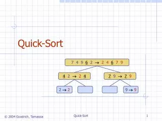
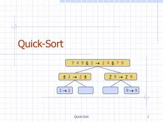
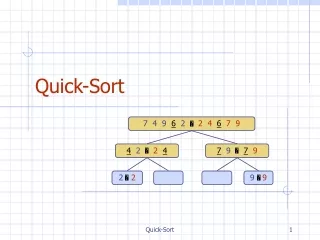
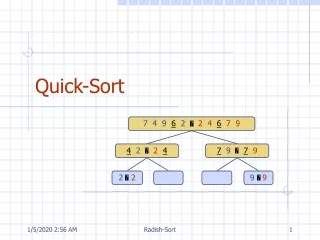
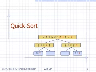
7 4 9 6 2 2 4 6 7 9 4 2 2 4 7 9 7 9 2 2 9 9 Quick-Sort Quick-Sort
Quick-sort is a randomized sorting algorithm based on the divide-and-conquer paradigm: Divide: pick a random element x (called pivot) and partition S into L elements less than x E elements equal x G elements greater than x Recur: sort L and G Conquer: join L, Eand G Quick-Sort (§ 10.2) x x L G E x Quick-Sort
Partition Algorithmpartition(S,p) Inputsequence S, position p of pivot Outputsubsequences L,E, G of the elements of S less than, equal to, or greater than the pivot, resp. L,E, G empty sequences x S.remove(p) whileS.isEmpty() y S.remove(S.first()) ify<x L.insertLast(y) else if y=x E.insertLast(y) else{ y > x } G.insertLast(y) return L,E, G • We partition an input sequence as follows: • We remove, in turn, each element y from S and • We insert y into L, Eor G,depending on the result of the comparison with the pivot x • Each insertion and removal is at the beginning or at the end of a sequence, and hence takes O(1) time • Thus, the partition step of quick-sort takes O(n) time Quick-Sort
Quick-Sort Tree • An execution of quick-sort is depicted by a binary tree • Each node represents a recursive call of quick-sort and stores • Unsorted sequence before the execution and its pivot • Sorted sequence at the end of the execution • The root is the initial call • The leaves are calls on subsequences of size 0 or 1 7 4 9 6 2 2 4 6 7 9 4 2 2 4 7 9 7 9 2 2 9 9 Quick-Sort
Execution Example • Pivot selection 7 2 9 4 3 7 6 11 2 3 4 6 7 8 9 7 2 9 4 2 4 7 9 3 8 6 1 1 3 8 6 9 4 4 9 3 3 8 8 2 2 9 9 4 4 Quick-Sort
Execution Example (cont.) • Partition, recursive call, pivot selection 7 2 9 4 3 7 6 11 2 3 4 6 7 8 9 2 4 3 1 2 4 7 9 3 8 6 1 1 3 8 6 9 4 4 9 3 3 8 8 2 2 9 9 4 4 Quick-Sort
Execution Example (cont.) • Partition, recursive call, base case 7 2 9 4 3 7 6 11 2 3 4 6 7 8 9 2 4 3 1 2 4 7 3 8 6 1 1 3 8 6 11 9 4 4 9 3 3 8 8 9 9 4 4 Quick-Sort
Execution Example (cont.) • Recursive call, …, base case, join 7 2 9 4 3 7 6 11 2 3 4 6 7 8 9 2 4 3 1 1 2 3 4 3 8 6 1 1 3 8 6 11 4 334 3 3 8 8 9 9 44 Quick-Sort
Execution Example (cont.) • Recursive call, pivot selection 7 2 9 4 3 7 6 11 2 3 4 6 7 8 9 2 4 3 1 1 2 3 4 7 9 7 1 1 3 8 6 11 4 334 8 8 9 9 9 9 44 Quick-Sort
Execution Example (cont.) • Partition, …, recursive call, base case 7 2 9 4 3 7 6 11 2 3 4 6 7 8 9 2 4 3 1 1 2 3 4 7 9 7 1 1 3 8 6 11 4 334 8 8 99 9 9 44 Quick-Sort
Execution Example (cont.) • Join, join 7 2 9 4 3 7 6 1 1 2 3 4 67 7 9 2 4 3 1 1 2 3 4 7 9 7 1779 11 4 334 8 8 99 9 9 44 Quick-Sort
Worst-case Running Time • The worst case for quick-sort occurs when the pivot is the unique minimum or maximum element • One of L and G has size n - 1 and the other has size 0 • The running time is proportional to the sum n+ (n- 1) + … + 2 + 1 • Thus, the worst-case running time of quick-sort is O(n2) … Quick-Sort
Consider a recursive call of quick-sort on a sequence of size s Good call: the sizes of L and G are each less than 3s/4 Bad call: one of L and G has size greater than 3s/4 A call is good with probability 1/2 1/2 of the possible pivots cause good calls: 1 2 3 4 5 6 7 8 9 10 11 12 13 14 15 16 Expected Running Time 7 2 9 4 3 7 6 1 9 7 2 9 4 3 7 6 1 1 7 2 9 4 3 7 6 2 4 3 1 7 9 7 1 1 Good call Bad call Bad pivots Good pivots Bad pivots Quick-Sort
Probabilistic Fact: The expected number of coin tosses required in order to get k heads is 2k For a node of depth i, we expect i/2 ancestors are good calls The size of the input sequence for the current call is at most (3/4)i/2n Expected Running Time, Part 2 • Therefore, we have • For a node of depth 2log4/3n, the expected input size is one • The expected height of the quick-sort tree is O(log n) • The amount or work done at the nodes of the same depth is O(n) • Thus, the expected running time of quick-sort is O(n log n) Quick-Sort
In-Place Quick-Sort • Quick-sort can be implemented to run in-place • In the partition step, we use replace operations to rearrange the elements of the input sequence such that • the elements less than the pivot have rank less than h • the elements equal to the pivot have rank between h and k • the elements greater than the pivot have rank greater than k • The recursive calls consider • elements with rank less than h • elements with rank greater than k AlgorithminPlaceQuickSort(S,l,r) Inputsequence S, ranks l and r Output sequence S with the elements of rank between l and rrearranged in increasing order ifl r return i a random integer between l and r x S.elemAtRank(i) (h,k) inPlacePartition(x) inPlaceQuickSort(S,l,h - 1) inPlaceQuickSort(S,k + 1,r) Quick-Sort
In-Place Partitioning • Perform the partition using two indices to split S into L and E U G (a similar method can split E U G into E and G). • Repeat until j and k cross: • Scan j to the right until finding an element > x. • Scan k to the left until finding an element < x. • Swap elements at indices j and k j k (pivot = 6) 3 2 5 1 0 7 3 5 9 2 7 9 8 9 7 6 9 j k 3 2 5 1 0 7 3 5 9 2 7 9 8 9 7 6 9 Quick-Sort
Summary of Sorting Algorithms Quick-Sort
Java Implementation public static void quickSort (Object[] S, Comparator c) { if (S.length < 2) return; // the array is already sorted in this case quickSortStep(S, c, 0, S.length-1); // recursive sort method } private static void quickSortStep (Object[] S, Comparator c, int leftBound, int rightBound ) { if (leftBound >= rightBound) return; // the indices have crossed Object temp; // temp object used for swapping Object pivot = S[rightBound]; int leftIndex = leftBound; // will scan rightward int rightIndex = rightBound-1; // will scan leftward while (leftIndex <= rightIndex) { // scan right until larger than the pivot while ( (leftIndex <= rightIndex) && (c.compare(S[leftIndex], pivot)<=0) ) leftIndex++; // scan leftward to find an element smaller than the pivot while ( (rightIndex >= leftIndex) && (c.compare(S[rightIndex], pivot)>=0)) rightIndex--; if (leftIndex < rightIndex) { // both elements were found temp = S[rightIndex]; S[rightIndex] = S[leftIndex]; // swap these elements S[leftIndex] = temp; } } // the loop continues until the indices cross temp = S[rightBound]; // swap pivot with the element at leftIndex S[rightBound] = S[leftIndex]; S[leftIndex] = temp; // the pivot is now at leftIndex, so recurse quickSortStep(S, c, leftBound, leftIndex-1); quickSortStep(S, c, leftIndex+1, rightBound); } only works for distinct elements Quick-Sort